 photometric sensitivity
at J, H, Ks in unconfused regions
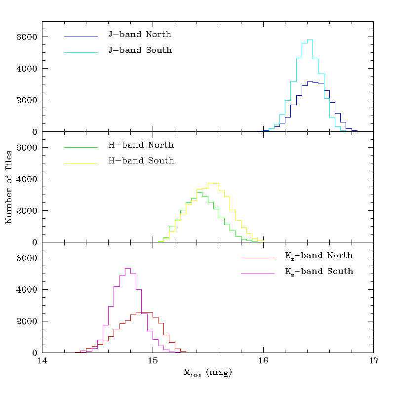
50% of coverage better than 16.4, 15.5, 14.8 mag
Most sensitive coverage at 16.8, 16.0, 15.3 mag
for any point on the celestial sphere
Hipparcos reference frame for [jhk]_m < 13.5 mag
)
The 2MASS All-Sky Point Source Release contains 470 million source extractions with a broad range of photometric quality. Various flags (rd_flg, cc_flg, bl_flg, ph_qual, prox, ext_key) permit users to distinguish between sources with reliable photometry and sources with suspect and/or poor photometry. The subsections below describe the overall nature and quality of the Point Source data and provide guidance for selecting reliable samples.
N.B.: The 2MASS All-Sky Point Source Release is deceptively named. "Point Source" refers to the fact that the fluxes and other parameters were extracted by 2MASS point source processing software. In the vast majority of cases, sources were indistinguishable from the system point-spread function (PSF) and the fluxes are valid point source flux estimates. In a small fraction of cases (about 1.6 million of the 470 million sources in the Release), the source profile was larger than the telescope PSF, indicating that the source was extended. Point source profiles fit to an extended profile produced an underestimate of the source flux. These same sources were detected and processed by the 2MASS extended source processor and form the basis of the 2MASS Extended Source Catalog. In the Point Source Release these sources have the ext_key flag set to the corresponding counter number in the Extended Source Catalog. Correct fluxes for extended sources can be found there. Queries seeking reliable point source photometry should exclude sources with non-null values of ext_key: (SQL: ext_key is null).
The admonition above is but one of several characteristics of the Release dataset which could produce misleading results for an uninformed user. The table below (as well as the discussion of the Point Source "caveats" (I.6.b) highlights several similar "traps" which could result in an embarrassing referee's report.
| Dynamic Range | >20 magnitudes (-4 through 16 mag at Ks) |
| 10 photometric sensitivity at J, H, Ks in unconfused regions | 100% of coverage
better than 15.9, 15.0, 14.3 mag 50% of coverage better than 16.4, 15.5, 14.8 mag Most sensitive coverage at 16.8, 16.0, 15.3 mag |
| Photometric Precision | [jhk]_cmsig < 0.03 mag for bright ([jhk]_m < 13.0 mag) stars |
| Photometric Uniformity | < 2% maximum photometric bias for any point on the celestial sphere |
| Astrometric Accuracy | <100 mas absolute
relative to the Hipparcos reference frame for [jhk]_m < 13.5 mag |
| Completeness | > 99% for ph_qual="A" sources
(i.e. >10) |
| Reliability | > 99.95% for ph_qual="A" sources |
2MASS photometry has a dynamic range of >20 magnitudes, owing to extraction software that address three different exposure regimes. The Survey's nominal frame exposure time was 1.3 s, obtained by differencing two readouts of the NICMOS3 array separated by that time interval. Both readouts were independently recorded and saved for future processing. The first readout (often referred to as "Read_1" in subsequent sections) occurred 51 ms after array reset and represents an effective 51 ms exposure image. The second read ("Read_2") occurred 1.351 s after reset. The point source database includes a rd_flg flag, which distinguishes between different techniques for populating the "default magnitude" column for sources, depending on their level of saturation (all XSC photometry derives from the 1.3 s "Read_2-Read_1" difference). Since different techniques can be used in different wavelength bands for a given source, the rd_flg is a three-character flag with an independent value for each band, revealing the source of the default magnitude (i.e. j_m, h_m, or k_m) column in the Point Source Release database.
Rigorous evaluation of repeated photometry, and thus limiting
sensitivity, as a function of observing
conditions (primarily seeing and airglow background), permitted
assignment
of limiting sensitivity for each survey Tile, in the absence of confusion
(and re-observation of Tiles which fell below the Survey's requirements
for photometric sensitivity). The histograms shown in Figures
1 and 2
document the achieved 10 sensitivity for every
Tile in the entire sky in each band. Details of the sensitivity estimation
and distribution of sensitivity on the sky are given
in Section VI.2.
| 
|
| Figure 1 | Figure 2 |
| Statistical | Spatial (Ks-band) |
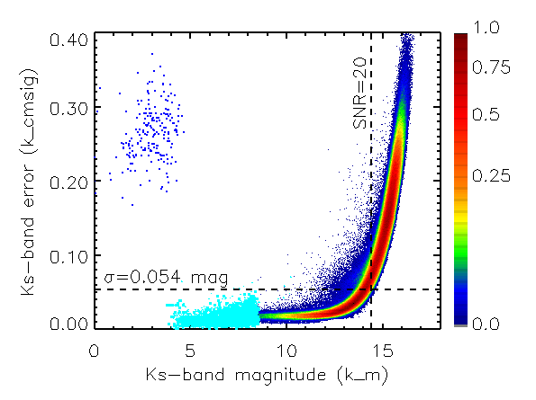
Repeated observations of sources provided empirical uncertainties, as a function of magnitude, as a means of validating the statistical uncertainties assigned to individual source by the extraction algorithms. The quoted default uncertainties are consistent with the repeatability statistics. Figure 3 illustrates the locus of quoted default uncertainty ([jhk]_cmsig) for Ks-band sources across the entire dynamic range of 2MASS. At faint magnitudes (Ks>13 mag) uncertainties rise, due to the dominance of background noise. For 8.5 < Ks (mag) < 13 default uncertainties are consistently in the range 0.02-0.03 mag. This limiting profile-fit uncertainty is attributable to undersampling, due to the coarse pixel size of 2MASS (2.0´´), relative to the seeing-limited image size (typically 1.0´´). Stars with 4 < Ks (mag) < 8.5 saturated in the 1.3 s duration 2MASS primary exposure. They were measured in the 51 ms "Read_1" exposure and extracted using aperture photometry receiving rd_flg=1. As a result, their mean uncertainties (light blue points) are slightly smaller than the profile-fit extractions. Stars with Ks < 4 mag saturated even in the 51 ms exposure. Their fluxes were extracted with a procedure that fit to the scattered light wings of the stellar profile. Figure 3 shows the substantially larger uncertainty associated with this procedure. The actual magnitude boundaries between these regimes vary with seeing and background conditions. Users should consult the rd_flg to track the origin of photometry for a given source. Details of the photometric extraction process and assignment of uncertainties are found in Sections IV.4.b and IV.4.c.
|
| Figure 3 |
Nightly/hourly calibration errors in 2MASS were estimated to be of order 0.01 mag (see IV.8). In addition, large scale drifts in the 2MASS photometric system were minimized (and evaluated) using a global photometric procedure, which calculated a simultaneous optimization of all available calibration measurements. Comparison of these solutions, obtained independently between hemispheres, shows <1% bias in the photometric calibrators around the sky (see the Photometric Uniformity analysis in VI.1).
Internal comparison of repeated 2MASS observations, and external comparison with more precise astrometric catalogs have demonstrated that the limiting astrometric accuracy of 2MASS is 100 milliarcseconds (mas) relative to the Hipparcos/Tycho coordinate system. The Astrometric Accuracy analysis in VI.1 addresses these comparisons in detail.
Some of the 1° × 8.5´ 2MASS calibration fields were
observed thousands of times during the course of the Survey. The
recoverability of stars in these fields, as a function of magnitude,
provides a definitive characterization of the Survey's completeness
statistics. There are sufficient trials that these statistics can
binned as a function of 10 limiting magnitude,
providing a means of selecting uniform samples at specified completeness
levels, as discussed in subsection II.2b.6 below.
Reliability has been assessed through
In both cases, reliability for sources which contain an "A" for the ph_qual flag (i.e., Catalog-level sources) exceeds 99.97% in all bands. A number of known sources of unreliability have been identified and excised from the Catalog (for example, bright star artifacts, hot pixels, and meteor trails). Less egregious examples of these phenomena survive, but contribute fewer than 0.03% of sources at the Catalog level. Despite this stringent reliability, a few hundred thousand unreliable sources lurk in the Catalog of nearly 0.5 billion objects. The Reliability analysis of VI.1 details the evaluation of reliability and known sources of unreliability.
ii. Accessing the 2MASS Point Source Release
The Infrared Processing and Analysis
Center (IPAC) processed the 2MASS images
and produced Catalogs of Point and Extended sources. These Catalogs,
which include photometry, astrometry, and an extensive set of quality
flags, are or will soon be publicly available from the following sources:
iii. Accessing the 2MASS J, H, and Ks Images
Discussion of 2MASS Point Source data would not be complete without
highlighting the available Images which underlie the Catalogs. The
Images are resampled to a common pixel scale and registered to a
common center, to aid in the production of color images and mosaics.
The images were generated by summing the six-deep, overlapping 1.3 s Survey
exposures. Most rd_flg=1 and all rd_flg=3 sources will
be saturated in these images, despite having useful flux extractions
in the Catalog.
iv. Basic Database Queries
Before attempting work with 2MASS Point Source data, users should read the
Point Source Cautionary Notes (I.6b) in detail and
familiarize themselves
with the explicit contents of the columns provided in the Release
(II.2.a).
The GATOR
website provides its own "user's
guide" and tutorial,
which provide specific examples of how to query the 2MASS Point Source
database using the IRSA GATOR interface. In addition to a general
user interface, the GATOR server permits queries based on Structured Query
Language (SQL). Below are a few introductory examples. The SQL
given in these examples can be inserted into the "User Defined
Constraints"
section on the GATOR query page (after removing the word "where,"
which is already assumed).
2MASS coordinates are in decimal degrees. GATOR provides an efficient "cone
search" utility for selection of sources within a 1°
radius of a central position as well.
This query rejects any source that has an E,F,U or X in
any of the three positions in the ph_qual flag.
In brief,
One should note that the restriction
rd_flg='002' means that the source was a profile-fit detection at
Ks and was not detected at J and
H (and the J and H default magnitudes contain upper
limits for the flux at this position, which might be used
in refining such a query). Technically, there might be a few
instances of very bright (Ks<9 mag) sources which appear as
rd_flg='001', but, for simplicity, they are not included in this
example. The query also tests that the Ks position in the
ph_qual flag does not contain a character indicating that the
photometry is suspect.
The first statement above selects sources with photometric
uncertainty lower than an explicit value in all three bands
(0.05 mag in this case).
The second statement makes use of the "photometric quality" flag
(ph_qual).
This flag, which contains one character for each Survey band,
contains "A" for sources which have both a scan signal to noise
ratio greater than 10 and [jhk]_cmsig<0.1086.
One should be aware that selecting ph_qual='AAA' or
[jhk]_cmsig<0.05 can produce a sample that is not
necessarily
statistically uniform. For "blue" (J-K<1.5 mag) sources
the uncertainty limits exclude sources based largely on the Ks-band flux.
For "red" sources the uncertainty limits exclude sources based on
their J-band flux. The resulting sample is a hybrid of J-band- and
Ks-band-limited selection. For applications, for example, where the
completeness must be well defined, uncertainty/ph_qual restrictions
should be applied to a single band (e.g., where ph_qual is
'A__').
The cc_flg
reports the likelihood of photometric contamination by nearby
bright stars or other image artifacts. The flag gal_contam is set
to a
non-zero value if the flux of the source lies within the 20
mag arcsec-2 elliptical isophote of an extended source.
The Catalog also contains a proximity column, which records the
distance to the nearest adjacent 2MASS source. A more restrictive
selection could require sources have prox>8.0,
since, for fainter sources, an adjacent faint star can also affect photometry.
N.B.: HOWEVER, there is significant danger in excluding
sources, using these
criteria when source densities are high. At high source density
virtually every source will be contaminated, and the resulting selection will
be a sparse representation of the Catalog contents
(see below).
Note that a source with ph_qual="A" is not a sufficient condition for
avoiding confused sources. BOTH cc_flg and ph_qual must be
consulted. A photometrically-contaminated source, according to
cc_flg, can still receive photometric quality "A".
v. Potential Hazards
All indications are that, within the Catalog subset of the
2MASS Point Source Release (i.e., those sources which contain an "A" in
the ph_qual flag and have use_src=1), the reliability exceeds
99.95%.
Only one in 2000 sources, at most, is an artifact. Still, in a
Catalog
containing 0.5 billion objects, this stringent reliability requirement
allows for more than 200,000 unreliable sources. Many of the
unreliable sources discovered and excised during the catalog
generation
process were single-band sources. Single-band sources in
the Catalogs should be regarded with suspicion -- even if all
flags indicate that the source is otherwise uncontaminated. Cosmic
ray events and hot, or unstable, pixels just below the exclusion
threshold could be retained in the Catalog as single-band sources.
At the same time, the Catalog is known to contain many astrophysically
valid single-band sources. The J-band channel of 2MASS was the most
sensitive to objects with J-Ks < 1.5 mag. Single-band "J-only"
sources will be common at high galactic latitude, where they represent
faint stars and galaxies just at the Survey's detection limit.
Conversely, intrinsically red objects (J-Ks > 1.5 mag) are more
favorably
detected in the Ks band. High-latitude active galactic nuclei and
L-type dwarfs, and
reddened objects at low latitude, are sources of "Ks-only"
detections. "H-only" detections should be regarded with
high suspicion, as they should trigger either a J- or Ks-
band detection as well. Values of [jhk]_psfchi significantly
in excess of 1.0 are indicative of poor profile fits and
may provide an additional indicator of an unreliable source.
The Point Source Cautionary Notes (I.6b) contains the most detailed account
of potential pitfalls encounted in using 2MASS data.
The subsections below highlight several critical examples.
The Point Source Catalog contains sources extracted using the
2MASS pipeline point source processing algorithms. A small
fraction of the sources in the Point Source Catalog (0.3%) are objects
recognized as extended sources by the pipeline extended source
processor. The point source algorithm will likely deliver an
underestimated
flux for such objects, since their shapes are broader than the system PSF.
Poor profile-fit extractions will be recognizable by
profile-fit
Stars dominate the Point Source Catalog, but, even after excluding
known extended sources, unresolved galaxies constitute a
non-negligible fraction of the PSC. In total, about 1% of the PSC
consists of unresolved galaxies. The unresolved galaxies are most
prominent at faint magnitudes (Ks > 14.0 mag) and red colors
(J-Ks > 1.0 mag).
In this color-magnitude regime unresolved galaxies can dominate stars
(see Figure 29 below).
Unresolved galaxies are likely to thwart purely color-selected
searches for, e.g., L-type dwarfs, at the flux limits of the Catalog.
While the 2MASS Point Source Catalog is designed to contain highly reliable
sources with accurate photometry, in some instances the photometry may be
suspect, even if the source was detected with a high signal to noise ratio.
The cc_flg indicates which sources
have a priori
suspect photometry and the reason why the photometry has been flagged.
If the cc_flg is not equal to '000' for a given source, then the
photometry
should be treated as suspect, in that systematic photometric errors may exist
which are not reflected in the quoted uncertainties from the 2MASS Point Source
Catalog. These systematic errors may result from contamination from a nearby
bright star, a diffraction spike, a persistence artifact, and other sources
described in Section
I.6.b. In addition, while the 2MASS Catalog meets a
high level
of reliability, there is an increased, but small, probability that a source
with a cc_flg not equal to '000' is an artifact. Therefore, before assigning
any special significance to a source based on the 2MASS photometry, it is
imperative that the cc_flg be examined (in addition to all other flags present
in the Point Source Catalog!) to determine if the photometry has been flagged
as suspect.
Given the above considerations, one may be tempted to exclude all sources
where the confusion flag (cc_flg) is not equal to '000', in order to extract the most
pristine set of point sources. While this procedure is acceptable for many
applications, it also compromises the completeness of the 2MASS Catalog.
In particular, crowded regions, such as the Galactic Plane or globular clusters,
can have a significant fraction of the stars flagged as confused, due to the
high source density. The globular cluster 47 Tucanae provides a
striking example (Figure 4).
Stars near the 1.3 s exposure limit of 2MASS and brighter produce
sufficient artifact and photometric contamination that a
flux-dependent source exclusion radius surrounds brighter stars
(and may follow their diffraction spikes out to even larger radii).
Although many sources were extracted inside this radius, few, if any,
survived catalog selection. Figure 5
illustrates the complete distribution
of sources around a star with Ks=-0.5 mag. Users making surface
density maps
in limited regions should remain aware that an unseen
bright star outside a region of study could remove a slice of
sky within the region of relevance.
A query which selects sources based entirely on sky position
(e.g., where ra is between 102.0 and 106.0 and dec is between
-5.0 and -2.0, in decimal degrees)
will draw many sources where
the rd_flg
contains a "0" or "6" in one, or even two, positions. Apparently valid
magnitudes appear in the default magnitude columns for such sources,
but:
A small fraction of the sources in the 2MASS Catalog have vanishingly
small
flux uncertainties, particularly those associated with aperture
photometry. These small uncertainties arise when a statistical fluke
causes the six independent measurements of the star to all have nearly
the same magnitude and thus produces a vanishingly small standard
deviation. Given that there are hundreds of millions of opportunities
for this to happen in the Catalog, these small uncertainties are a
natural consequence of the statistical process and are to be expected.
The population uncertainty (see Figure 3)
for objects with similar flux will be much
larger and provides a more appropriate estimate of the flux uncertainty.
Large values of
2MASS magnitudes are reported in the intrinsic 2MASS photometric
system. That is, the reported fluxes are directly related to
the observed fluxes of the network of 2MASS standard stars.
Explicit color transformations (see VI.4b)
are available to many common near-infrared photometric systems.
As discussed in Section IV.4b, a PSF mismatched to
the seeing conditions can cause a photometric error of up to ~0.02 mag. For
most stars, this error is negligible compared to the photometric
uncertainty. However, when computing the average stellar color over a
region of the sky, and thereby computing a very accurate mean stellar
color, the systematic uncertainty due to the mismatched PSF may be
significant. This section illustrates the effects of a mismatched PSF
on the photometry, demonstrates one possible solution to minimize the
error using data available using GATOR, and
outlines steps to further improve the analysis.
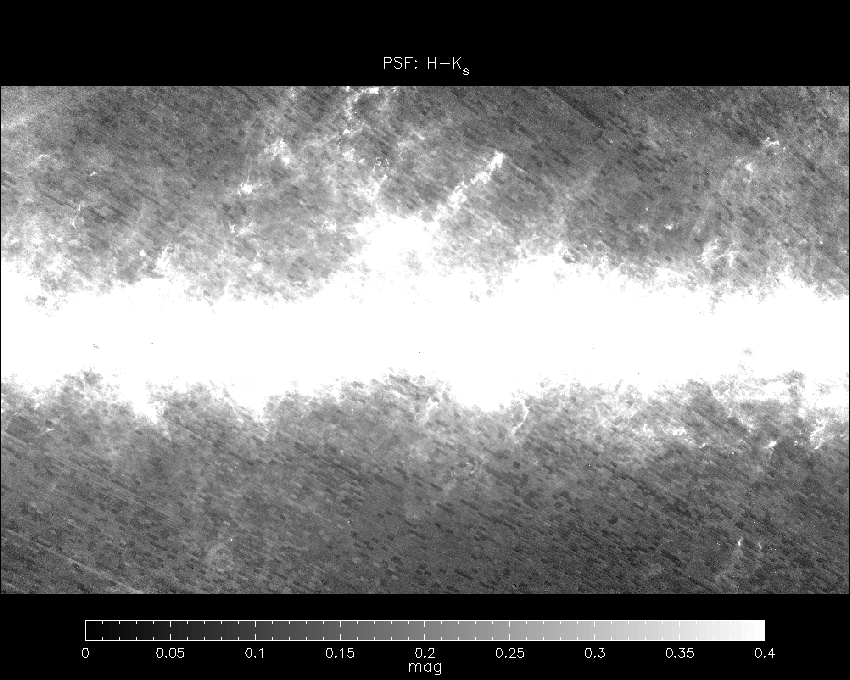
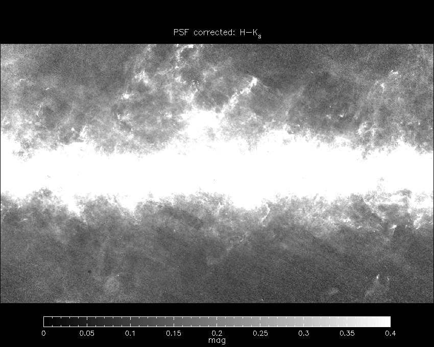
Figure 7 shows an image of the average
H-Ks color for 2MASS Point Sources toward the Galactic Center with
Ks
At high galactic latitudes, one discerns a rectangular grid pattern to the
distribution of H-Ks colors. These grids correspond spatially to
the individual 2MASS Atlas Images, and indicates that
the 2MASS data processing has introduced a color bias to the J, H, and
Ks photometry.
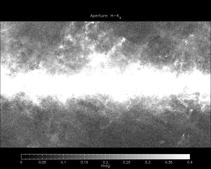
Figure 8 shows a similar image of the average
colors, but where the colors were computed using the aperture magnitudes.
(This figure contains many individual pixels where the colors deviate from the
surrounding average, which reflects the inherent difficulty in performing
aperture photometry in source-confused regions.) The rectangular grid pattern
is no longer evident when using the aperture magnitudes, and suggests that the
color biases seen in Figure 7 are due to
errors in the PSF photometry.
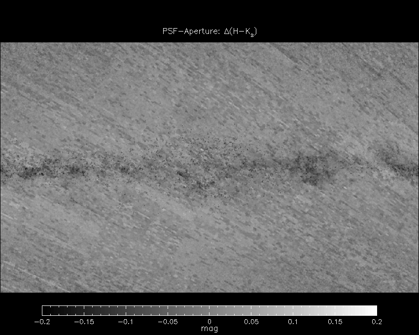
To quantify the amplitude of the color bias, the color map computed with
aperture photometry was subtracted from the PSF map. The difference image was
median filtered with a 3×3 pixel2 box (and using only pixels with color
differences less than 0.25 mag) to remove the highly deviant pixels.
The difference image (see Figure 9)
clearly shows the grid pattern found in the PSF photometry map. A histogram of
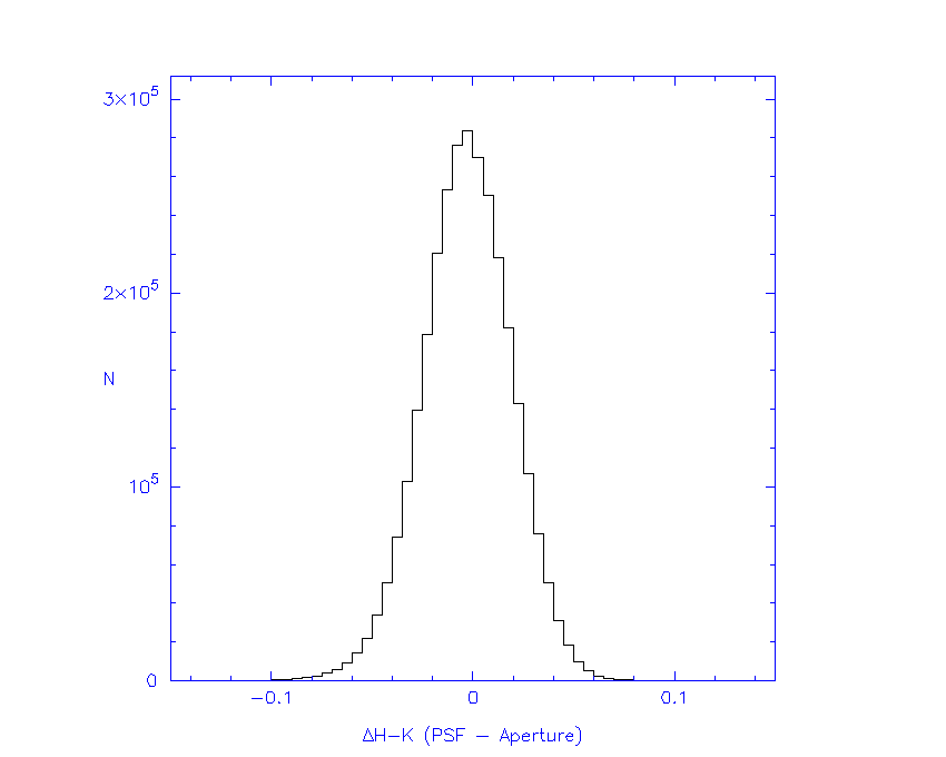
the color differences for galactic latitudes |b| > 1°
(Figure 10) indicates that the
RMS of the color bias in the difference image is 0.022 mag. The
difference image was used to apply a first-order correction to the PSF
photometry. The resulting H-Ks image (see
Figure 11) can be directly compared
to the original image (Figure 7) and shows
that the amplitude bias has been substantially reduced.
These color biases should be present at all galactic latitudes, but are only
clearly seen toward the Galactic Center, where the counting statistics are
sufficient to detect the small bias at the angular scale corresponding
to an individual 2MASS image. The prescription outlined here did not completely
remove the artifacts, but the analysis can be improved as follows:
The NASA/IPAC Infrared Science Archive
(IRSA) provides access to data from several NASA infrared and
submillimeter
missions through the
GATOR
catalog browser. The 2MASS Catalogs can be searched by
coordinates or
source name (in addition to more sophisticated queries), and
the
results downloaded as ASCII files.
Compressed files of the entire 2MASS Catalogs are
available for downloading via
anonymous ftp.
The compressed Point Source Catalog is 42.6 GB.
The 2MASS Project has produced a limited supply of DVD-ROMs
containing the 2MASS
results, including the Point Source Catalog, the Extended
Source Catalog. The DVDs do not contain Images.
The DVD-ROM set can be ordered by sending 2MASS an
email
with your name, institution, and full mailing address.
You should also
consult the All-Sky DVD Release Updates
for the most recent information on the DVD-ROMs.
The Centre de Donn
The 2MASS Image Atlas contains photometrically and
astrometrically
calibrated J, H, and Ks FITS-format images for the entire
sky. Each
Image in the Atlas has dimensions of 512 × 1024 pixel2,
with
1.00´´ pixels, to provide a field-of-view of
8.53´ × 17.07´. The J, H, and Ks Images are spatially
registered and have a common pixel scale.
Currently, lossy-compressed versions of the Images
(i.e., "Quicklook" images) are available through the
2MASS Quicklook Image Services, which is administered by
IRSA.
At a later date, lossless-compressed Atlas Images will be made
available
through
IRSA.
The images contain astrometric information using standard
FITS
keywords, and the magnitude zero points are also stored in the
FITS
headers. However, in most instances the photometry and
astrometry listed
in the 2MASS Point Source Catalog will be more accurate, since it
was
derived from the raw images. In addition, since the Quicklook
images
are restored from lossy-compressed files, they are not
recommended for photometric measurements (see the discussion of
Photometry from 2MASS Compressed/Uncompressed Images).
Both single Atlas Image and batch image downloads are available.
is not entirely sufficient to assure a reliable set of clean
detections,
because the ph_qual conditions cited above do occur
for rd_flg=1 and rd_flg=2 sources.
unresolved pairs of stars can trigger the  2
value was in excess of 10.0 or
2
criterion, in particular.
2
value was in excess of 10.0 or
2
criterion, in particular.
2 values ([jhk]_psfchi) substantially in excess of
1.0. Sources recognized as extended by the extended
source processor and appearing in the Extended Source Catalog
will have non-null values in the ext_key column of the Point Source
Catalog. This ext_key value is a cross reference to the matching
source in the XSC.
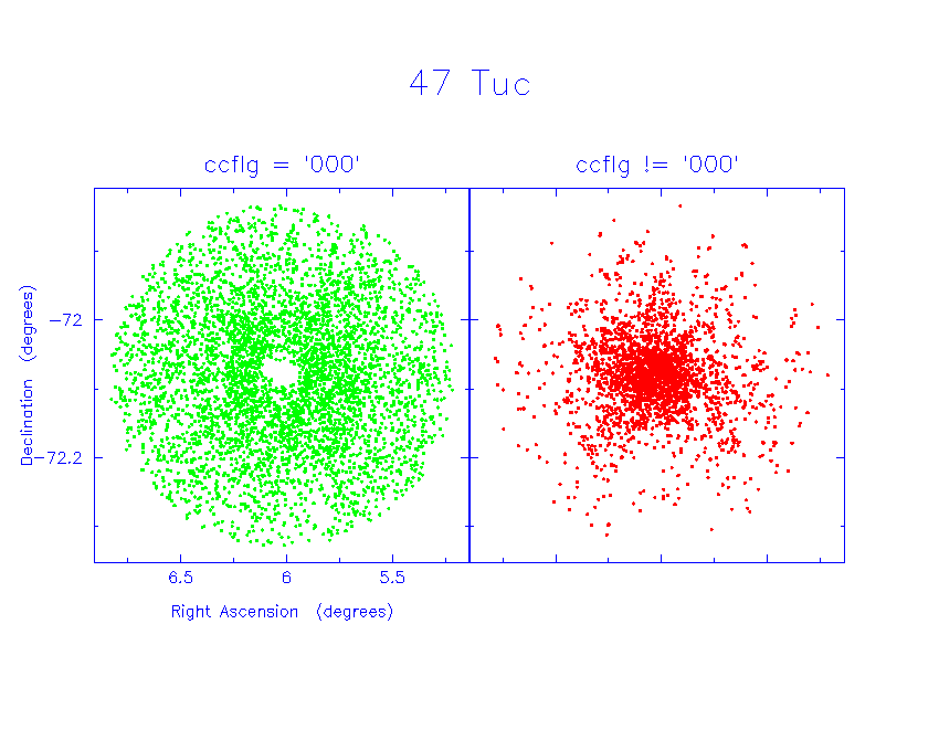
Figure 4
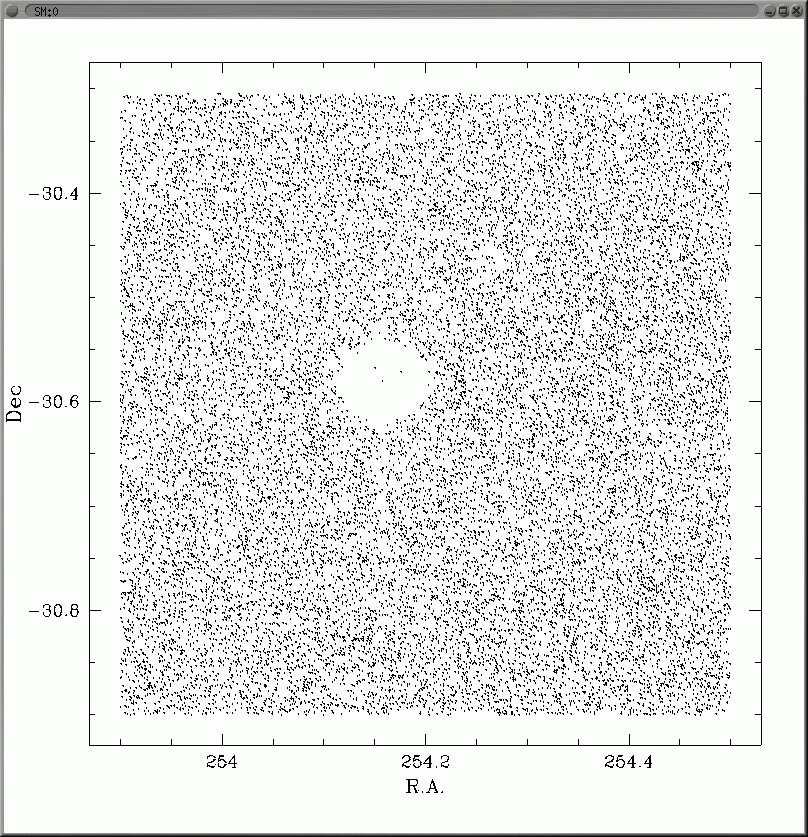
Figure 5
Either condition sets the ph_qual
flag to "U" for that band. Conversely, reliable three-band detections
of real flux can be obtained by requiring the ph_qual flag contain
an "A", "B", "C", or "D" (in order of increasing flux uncertainty) in
each of its three positions. This selection is best accomplished by
ruling
out all of the poor-quality variants of the ph_qual flag ( where ph_qual not
matches '[EFUX]' ).
as highly precise
measurements
2
([jhk]_psfchi) are statistically representative.
2 not only indicate a
poor fit for the profile-fit procedure, but also imply that the profile-fit
error model is not
a valid one for that particular source. Figure 6 shows the
difference between profile-fit and aperture magnitude, in units of
[jhk]_cmsig as a function of [jhk]_psfchi.
The flux underestimate
for large [jhk]_psfchi sources is evident as a larger scatter
in the normalized errors, indicating a poorer estimate of the flux
uncertainty.
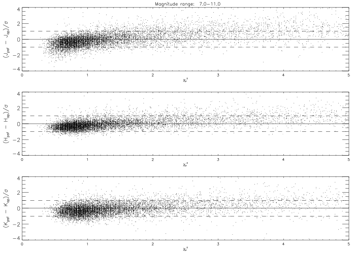
Figure 6  14.3 mag. The colors were computed using the default 2MASS
magnitudes, which for most sources represents photometry computed by fitting a
PSF to the 2MASS images. The high extinction associated with
the Galactic Plane is clearly visible as the horizontal band of red
H-Ks colors.
14.3 mag. The colors were computed using the default 2MASS
magnitudes, which for most sources represents photometry computed by fitting a
PSF to the 2MASS images. The high extinction associated with
the Galactic Plane is clearly visible as the horizontal band of red
H-Ks colors.
| H-Ks colors toward the Galactic Center | ||||
| PSF | Aperture | PSF-Aperture | Delta(H-Ks) Histogram | Empirical PSF correction |
|
|
|
|
|
| Figure 7 | Figure 8 | Figure 9 | Figure 10 | Figure 11 |
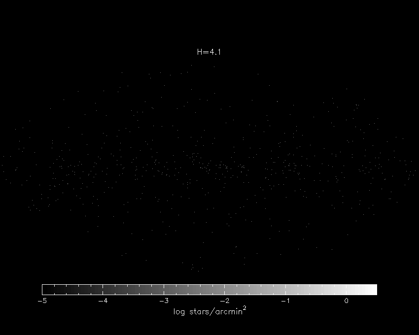
vi. Obtaining Uniform Samples over Large Areas
The two figures below compare stellar density in two narrow J-band
magnitude slices. Figure 12 is from a magnitude range (J
= 15.8--16.0 mag), where the Survey is 99% complete for virtually all of the
sky. Little, if any, imprint of the Survey scan pattern is evident.
Figure 13 shows J-band source counts from a J-band
magnitude range that is 0.8 mag fainter (J = 16.6--16.8 mag). In
this faint magnitude range the stellar density is biased
by the survey Tile pattern, because of the varying sensitivity of the
Survey, driven primarily by airglow and seeing. Conversely, this
figure indicates that large contiguous regions of the sky are complete to
flux levels as much as a magnitude fainter than the nominal 2MASS
completeness limits.
Uniformity in Unconfused Regions
| 
|
| Figure 12 | Figure 13 |
| 15.8<j_m<16.0 | 16.6<j_m<16.8 |
The 10 sensitivity limit, computed for
every individual Tile, based on seeing, background, and calibration
zeropoint, provides a guide to selection of flux limits which provide
uniform catalogs over steradian scales and selection of modest
contiguous areas of the sky, which are complete at fainter magnitudes.
2MASS tracked sensitivity empirically as a function of observing conditions,
by monitoring the statistics of repeated observations of sources
under varying conditions of seeing and background
(see VI.2). The repeated
observations, in this case, were Survey calibration observations
which occurred several times each night. Each calibration observation
consisted of six independent observations of every star in a 1° ×
8.5´ field. Assessing the flux uncertainty empirically
from the standard deviation of the repeated measurements
permitted an estimate of uncertainty vs. flux for the instantaneous
seeing, airglow, and system zeropoint which prevailed at the time of
observation. Collecting these observations from the range of
conditions encountered during the three-year history of observations
yielded a means of characterizing the sensitivity of any independently-observed
Survey Tile using these key variables. In fact, many Survey Tiles
were re-observed when the conditions indicated that the Tile's
sensitivity fell below the Survey's sensitivity specification.
Virtually the entire sky was observed at least once with sensitivity
at or better than Survey specifications as a result. The 10
limiting sensitivity of each Survey scan is quantified in a column of the
ancillary Scan Information Table.
The Survey's thousands of repeated calibration observations also
provided a means of assessing the Survey's completeness as a function
of magnitude, simply by tracking the number of times a given source
was detected, compared with the number of opportunities for detection.
Since calibration observations were obtained over a broad range
of 10 limiting sensitivity, these empirical
completeness statistics can be binned by sensitivity.
Figure 14 shows that the empirical
completeness percentage declines steeply
faintward of the 10 sensitivity threshold and
scales
faintward as expected with limiting 10 magnitude.
The table below provides guidance on
setting a completeness limit vs. the 10 magnitude for any given
Tile, based on the data in Figure 14.
99% or better completeness can be obtained for
the entire unconfused sky by selecting sources with a
limit 0.1 magnitude brighter than the poorest 10-limiting
sensitivity in the histogram in Figure 1 -- or 15.9, 15.0, and 14.2 mag
at J, H, and Ks, respectively.
| Achieved Completeness | > 50% | > 80% | > 90% | > 95% | > 99% |
| Completeness threshold for10 magnitude=M |
M+0.20 | M+0.10 | M+0.05 | M-0.05 | M-0.10 |
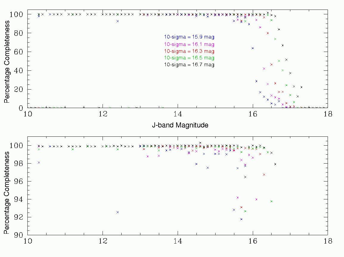
|
| Figure 14 |
In addition to appropriate flux limits, use of the "use_src" flag is important in obtaining truly uniform sampling of the sky. 2MASS Tiles overlap by a small amount. About 20% of the sky was observed two times or more as a result of this overlap. A selection algorithm has chosen a single apparition of each source with the potential for multiple observations, to remove any bias associated with multiple opportunities to observe a source (see V.4). If a source was observed only once in two opportunities, the algorithm would decide whether or not to include the source in the Catalog in an unbiased manner. Occasionally, bright sources would be missed on one of two apparitions, due to effects, such as one apparition falling on the persistence image of a nearby bright star. These bright sources are included in the Catalog for completeness, but should not be used when selecting uniform samples. The use_src flag permits this distinction. Sources selected with use_src=1 will be representative of a uniform 2MASS selection.
The complete thresholds described below pertain to unconfused regions of the sky. In high-source density regions, such as globular clusters or the Galactic Plane, confusion noise from unresolved point sources will limit the point source completeness and photometric accuracy. This subsection presents an empirical determination of the uniformity of the 2MASS Point Source Catalog in high density regions.
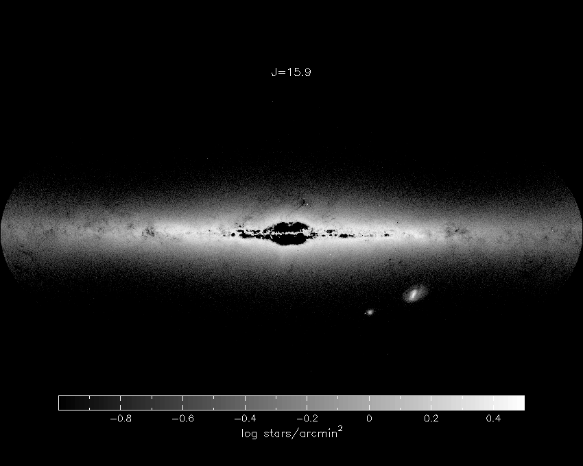
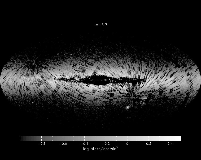
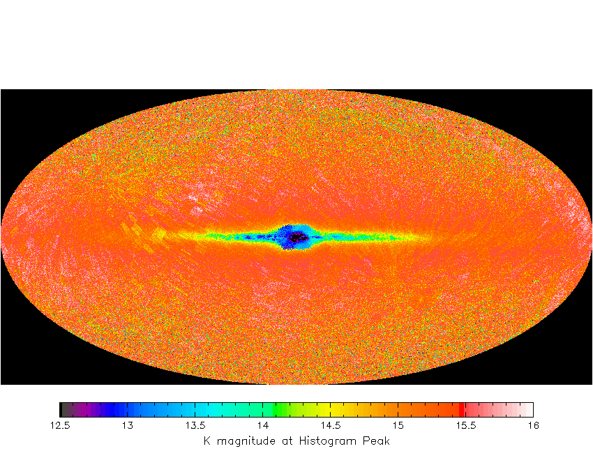
A simple, yet powerful, visual representation of the 2MASS completeness limit over the entire sky can be obtained by viewing the "movies" in Figures 15, 16, and 17. These movies cycle through images of the differential star counts, in 0.2 mag bins, presented in the Galactic Aitoff projection. The Galactic Plane is clearly visible in these movies as the bright horizontal band. The star count maps show a patchy distribution in the Galactic Plane, especially at J, due to extinction from dust within the Galaxy. Beginning at approximately J=14, H=13.5, and Ks=13 mag, the star count maps start developing holes (as represented by the black regions), first near the Galactic center, and expanding to larger galactic latitudes for fainter magnitudes. These holes are a result of confusion noise.
| GIF Movies of the 2MASS Sky | ||
| J-band | H-band | Ks-band |

|
|

|
| Figure 15 | Figure 16 | Figure 17 |
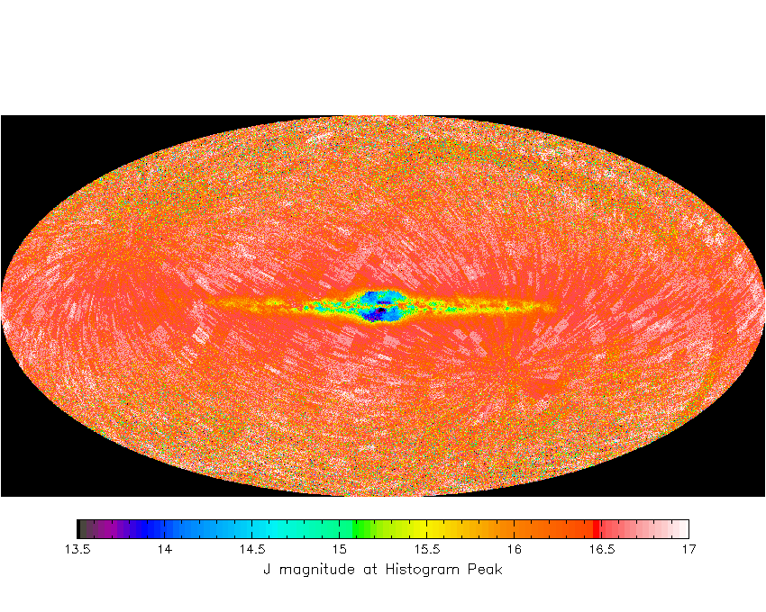
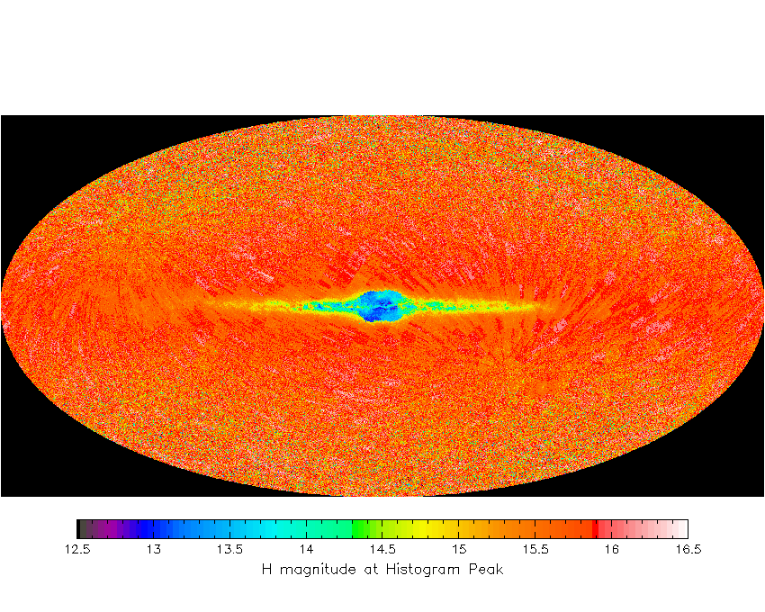
The above impressions where quantified by computing, for each 10 × 10 arcmin2 pixel in the star count maps, the magnitude bin which contains the peak star counts. The magnitude at the peak star counts was taken as a measure of the completeness. Note that this definition of completeness differs from that used to characterize the 2MASS Point Source Catalog, which was defined to be the faintest magnitude bin which recovers 99% of the expected source counts and was measured based on repeated observations of 2MASS calibration fields and overlap regions in the 2MASS survey. The definition of completeness used here is not as stringent.
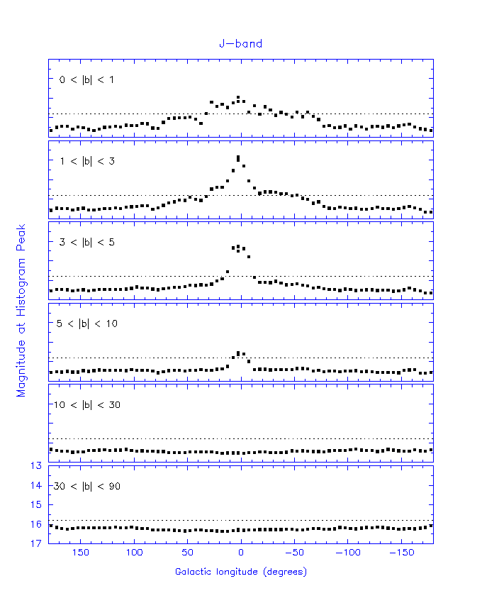
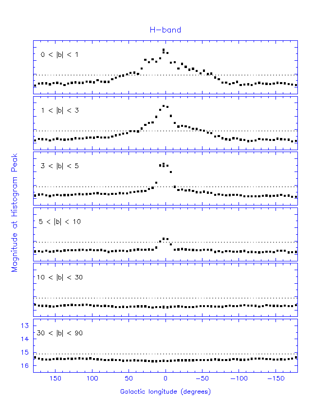
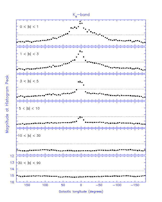
Figures 18, 19, and 20 show images of the derived completeness limits in the Galactic Aitoff projection for the J, H, and Ks bands. Further, Figures 21, 22, and 23 show the average completeness limit, as a function of galactic longitude, for several latitude bins. Relative to the average completeness at high galactic latitude (|b|> 30°), incompleteness in the Galactic Plane occurs within approximately (a) 80° of the Galactic Center for |b| < 3°, and (b) 6° of the Galactic Center.
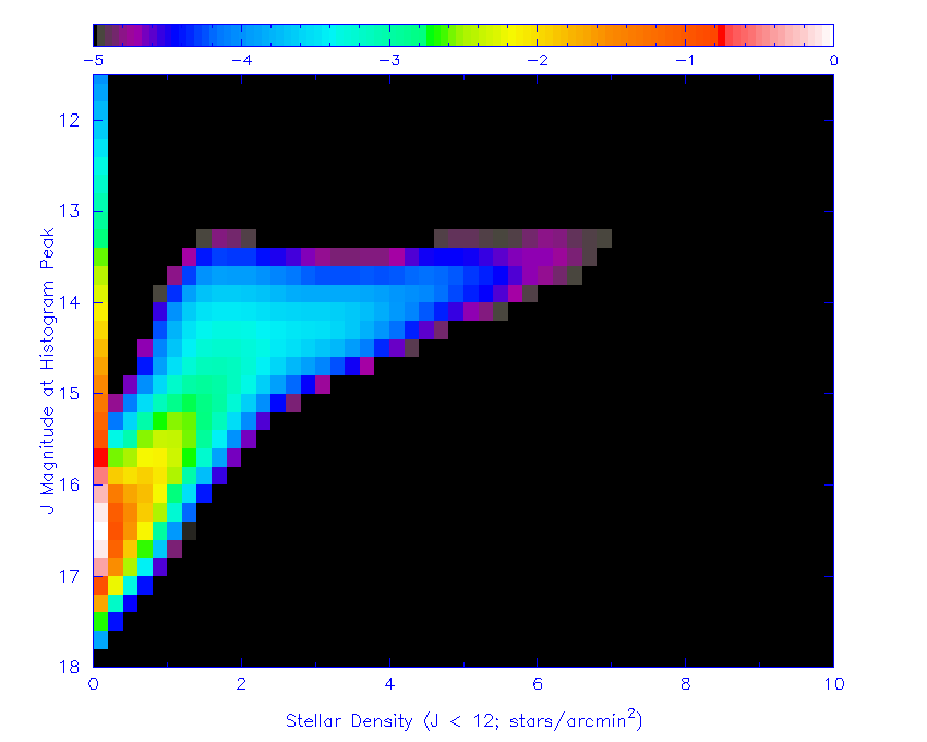
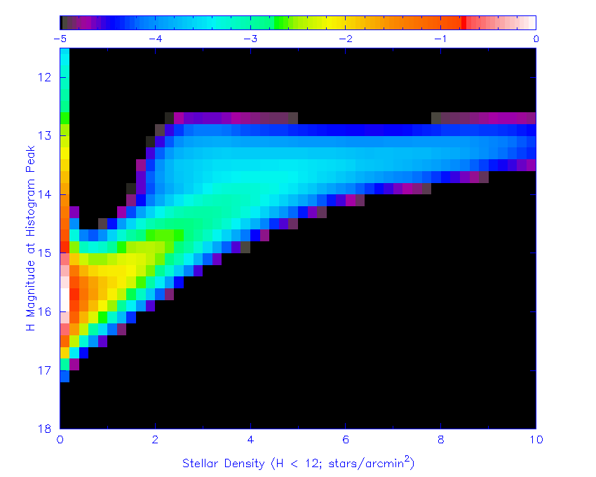
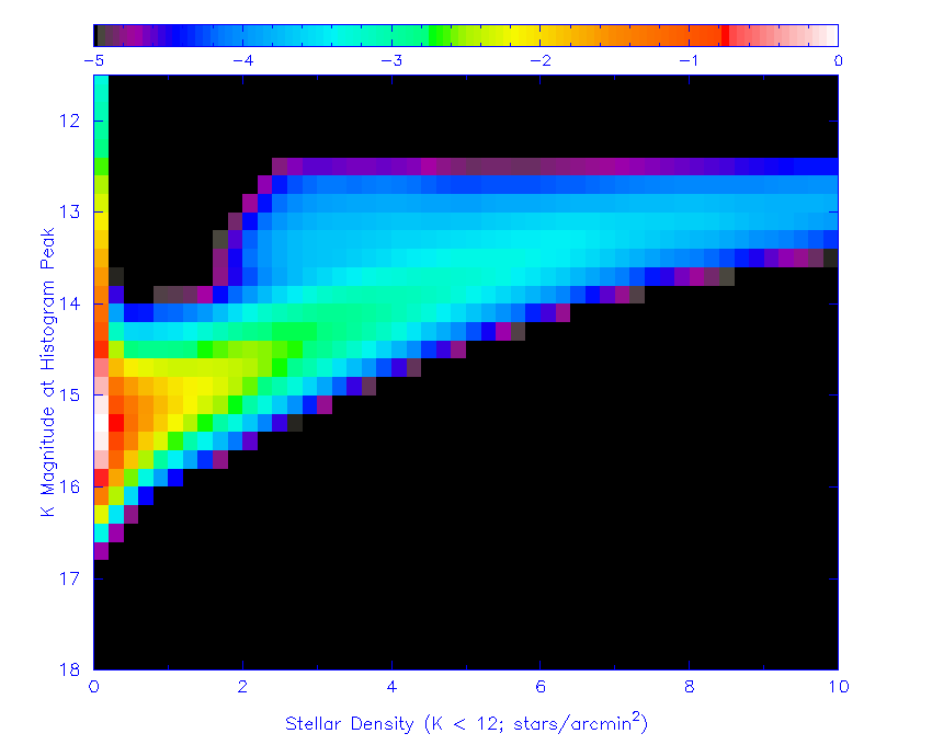
In addition to the Galactic Plane, the completeness limit will occur at bright magnitudes in high density regions, such as the Large Magellanic Cloud and globular clusters. For these regions, it is instructive to view the completeness limit as a function of source density. Figures 24, 25, and 26 show magnitude of the peak star count bin as a function of source density. The source density has been computed for sources brighter than magnitude=12, since Figures 18--23 indicate that nearly the entire sky is complete to that magnitude limit. The color scales in Figures 24, 25, and 26 are normalized such that peak value is unity. These figures show that at low stellar densities (i.e., high galactic latitudes), the magnitude histograms peak at approximately J=16.5, H=15.7, and Ks=15.2 mag. As the stellar density increases, the magnitude histograms systematically peak at brighter magnitudes.
|
|
|
| Figure 18 | Figure 19 | Figure 20 |
|
|
|
| Figure 21 | Figure 22 | Figure 23 |
|
|
|
| Figure 24 | Figure 25 | Figure 26 |
vii. Example Query Results
The subsections that follow present the results of increasingly
refined queries on the Point Source Release database,
aimed to produce source fluxes of the greatest accuracy and
astrophysical relevance.
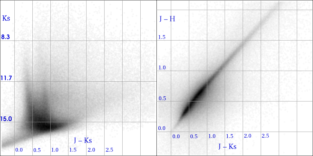
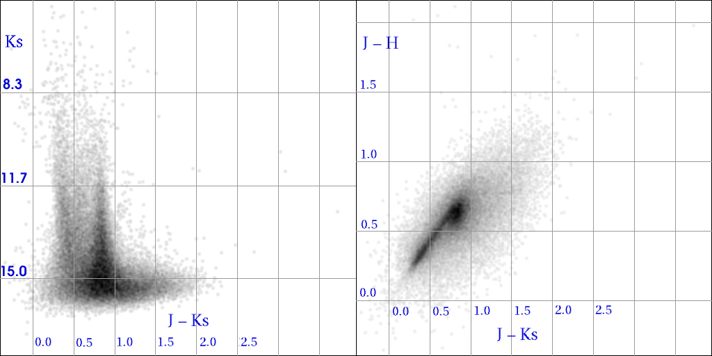
The color-color and color-magnitude diagram in
Figure 27
result from a random sampling of 0.1% of the 2MASS Release database.
Evident is a substantial smearing of the color-magnitude diagram, due
to Galactic reddening. This reddening appears as the narrow
spike extending toward the upper right in the
color-color diagram (demonstrating the relative uniformity
of the Galactic extinction law). Distinct features in the
color-magnitude diagram (seen in the figures in the subsection below) are
similarly smeared beyond recognition by reddening.
Photometric Characteristics of the Complete Dataset
|
| Figure 27 |
SQL: where abs(glat)>35.
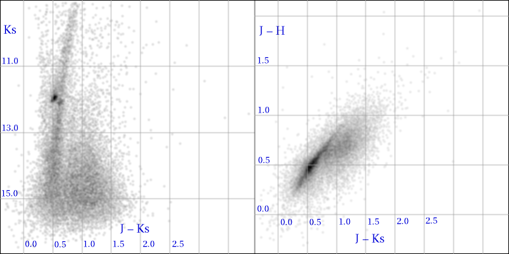
The effects of source density and reddening in the Galactic plane are discussed in detail in Section VI.7. Since the present subsection focuses on producing the highest quality photometry, subsequent examples address only high galactic latitudes, where reddening does not significantly bias stellar colors. The diagrams in Figure 28 show the results of selecting 2MASS sources at galactic latitude of 35° or more from the Galactic plane. The effects of reddening are no longer evident, and the distribution of stars in the diagram reflects true astrophysical colors of various stellar classes. This diagram, however, derives from all sources above the galactic latitude restriction, without regard for noisy detections (ph_qual), confusion (cc_flg), and upper limits (rd_flg). The colors of some of the sources are thus either contaminated or simply nonsense.
|
| Figure 28 |
SQL: where abs(glat)>35. and ph_qual not matches '[EFUX]'
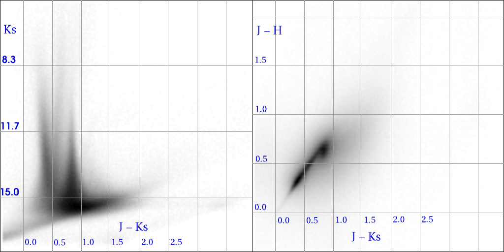
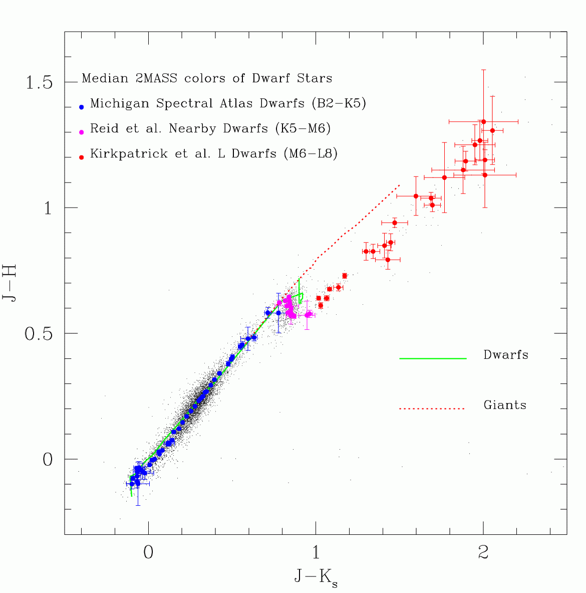
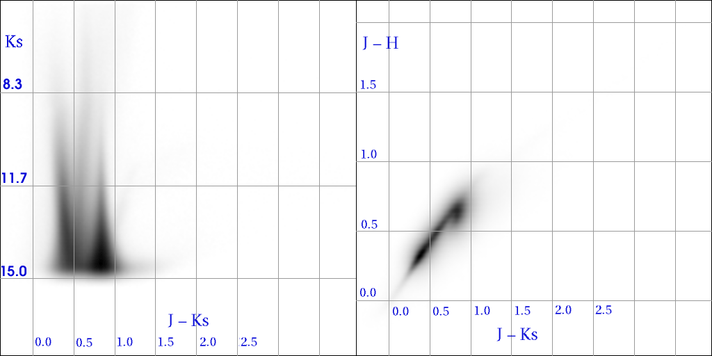
The diagonal features at faint magnitudes in the previous example arise from the use of upper limits calculated at the positions of non-detections. Sources must be detected in all three bands (and thus have a rd_flg value of 1, 2 or 3, in each rd_flg position) for valid color-color analysis. In addition, they must have valid photometric quality. All positions in the ph_qual flag must contain an "A", "B", "C", or "D". This condition is obtained by selecting against the other possible values of ph_qual that indicate non-existant or corrupted photometry ("E", "F", "U", and "X") The ph_qual restriction naturally delivers sources with valid rd_flg values. Figure 29, which includes only sources with valid three-band detections, is dominated entirely by astrophysical features convolved with the Survey's noise characteristics. The vertical spikes in the color-magnitude diagram are common dwarfs (left) and giants (right) smeared in apparent magnitude by their varying distance. The spikes are "sharp" at the bright end and broaden toward faint magnitudes, due to increasing flux uncertainty. In the color-color diagram the sources largely cluster along the coincident giant and main-sequence track for stars of earlier spectral type than K5. The "hook" at the red end of this distribution arises from K7/M0 main-sequence stars and cooler, which now deviate from the nearly linear trend (giants continue along the linear sequence as shown in Figure 30). The sources redder than J-Ks=1.0 mag at faint magnitudes are largely unresolved galaxies.
|
|
| Figure 29 | Figure 30 |
SQL: where abs(glat)>35. and ph_qual not matches '[EFUX]' and cc_flg='000' and gal_contam=0 and ext_key is null
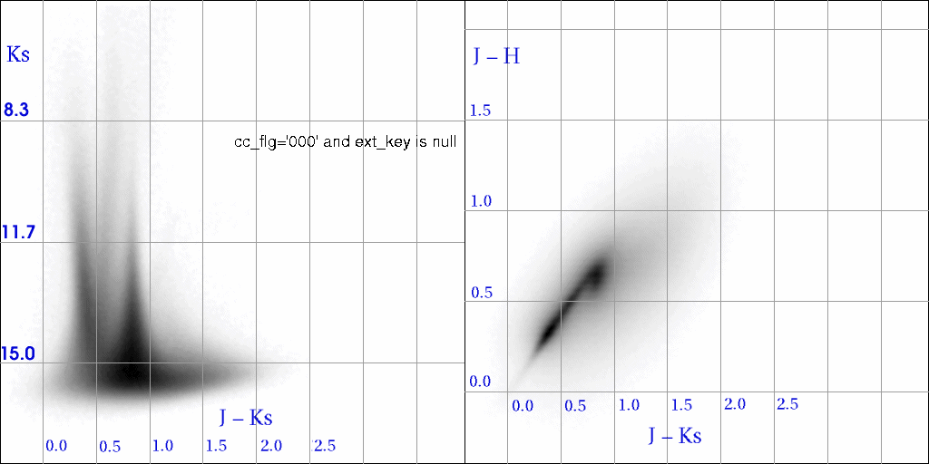
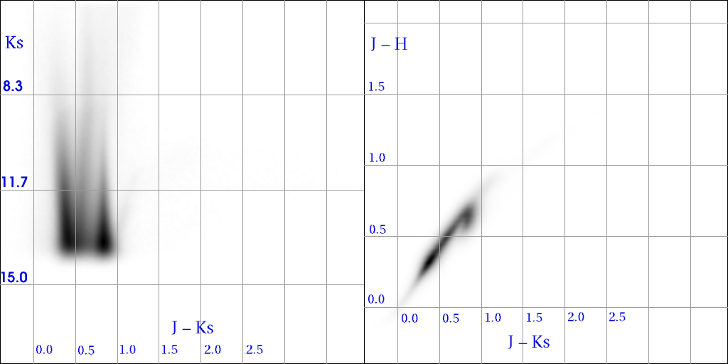
Contaminated photometry and extended sources must be eliminated in order to obtain the most photometrically pristine sample of stars. Point sources contaminated by nearby extended sources have gal_contam set to a non-zero value. The cc_flg is set to a value other than "0" in a given band when diffraction spikes ("d"), artifacts ("p"), or simply scattered light ("c") from an adjacent star potentially contaminate a source's flux. The value cc_flg="c" is set to flag sources whose flux is likely to be in error by 5% or more, due to flux contamination from a nearby star. (Alternatively, additionally requiring prox > 8.0, in arcsec, provides more conservative protection from contamination from close faint stars at the expense of eliminating significant portions of the sources in high density regions.) Figure 31 contains sources which have cc_flg='000' and gal_contam=0. Sources included in this plot also have "null" values in their ext_key column, indicating that they were not identified as an extended object by the extended source processing. Plenty of galaxies remain in the Point Source Release after this exclusion -- all unresolved. These unresolved galaxies form the faint red haze beyond the red end of the main sequence in the color-color diagram and the extended red pedestal at faint magnitudes in the color-magnitude diagram. Comparison with Figure 29 shows that the removed extended sources populated the brighter portion of the red extragalactic distribution (see Figure 32).
Figure 33 shows the result of an "inverse" query intended to select potentially contaminated objects. This diagram contains sources with prox < 8 and with non-zero values in the cc_flg. By and large, this "contaminated" sample resembles the "clean" sample in Figure 31, in part reflecting the conservative nature of the confusion flagging and in part indicating that flux contamination may have lesser influence on stellar colors. Given that a source is flagged as photometrically contaminated when the flux is likely biased by 0.05 mag, and given that the vertical scale in the color-magnitude diagrams spans more than 10 magnitudes, the fact that there is little obvious bias in the "contaminated" sample arises mainly from the small contamination needed to trigger the flag.
Figure 34 similarly shows sources that received gal_contam=2 indicating they were contaminated by a nearby extended source. Surprisingly, the diagram seems to contain obvious red giant branches and red clumps. This result occurs because globular clusters are identified as extended by the extended source processor, and many of their stars lie within the 20 mag arcsec-2 isophote used to set the gal_contam flag. In addition to these features, there is a significant haze of points in the red regions populated by galaxies, indicative of true extragalactic contamination.
 |
 |
 |
 |
| Figure 31 cc_flg='000' and gal_contam=0 |
Figure 32 "blink" vs. Figure 4 |
Figure 33 cc_flg!='000' or prox<8.0 |
Figure 34 gal_contam!=0 |
SQL: where abs(glat)>35. and ph_qual not matches '[EFUX]' and cc_flg='000' and gal_contam=0 and ext_key is null and ph_qual="AAA"
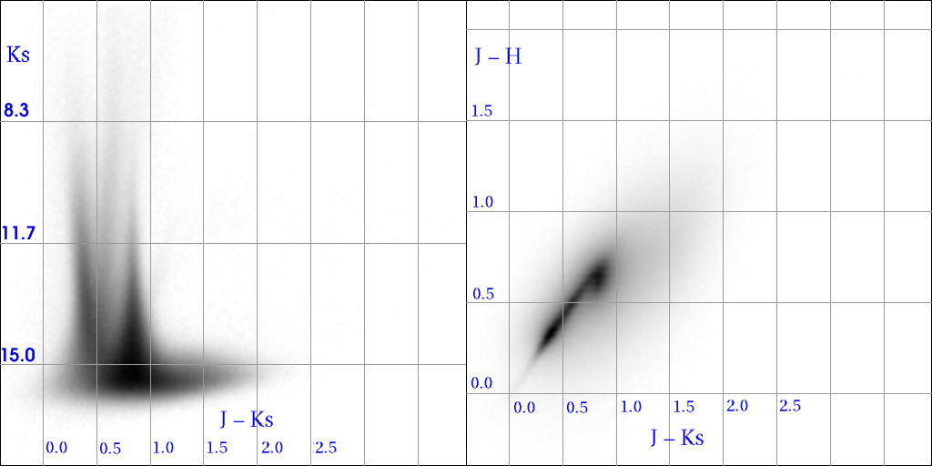
Since detection above SNR>7 in any one band or SNR>5 in two bands is sufficient to include all three bands of source extractions in the Release database, many sources may have exceptionally large flux uncertainties in some bands. The previous figures included sources with relatively low signal to noise ratio and, thus, large photometric uncertainty. A variety of means exists to select samples of sources with small photometric uncertainty. A very simple approach involves using the "photometric quality" flag -- ph_qual. This three-character (one for each band) flag is set to "A" in a given band when the photometric uncertainty for the source extraction is <0.109 mag and the source flux to sky noise ratio exceeds 10. Selecting sources with ph_qual="AAA" ensures modest uncertainty in all three bands (Figure 35). Most apparent in these figures is the absence of the wide pedestals in the color-magnitude diagram. Since SNR=10 is typically achieved at Ks~14.5 mag, fainter sources do not survive the ph_qual="AAA" restriction.
 |
| Figure 35 ph_qual="AAA" |
SQL: where abs(glat)>35. and ph_qual not matches '[EFUX]' and cc_flg='000' and gal_contam=0 and ext_key is null and j_msigcom<0.05 and h_msigcom<0.05 and k_msigcom<0.05
and
SQL: where abs(glat)>35. and ph_qual not matches '[EFUX]' and cc_flg='000' and gal_contam=0 and ext_key is null and j_msigcom<0.03 and h_msigcom<0.03 and k_msigcom<0.03
The large (2´´) 2MASS camera pixels limit the Survey's ultimate precision to about 0.02 to 0.03 mag. This level of precision is regularly achieved for sources not limited by other intrinsic noise sources. Figures 36 and 37 illustrate the result when the final combined uncertainty ([jhk]_msigcom) constrains the sample selection. The samples do not extend to as faint a magnitude in the color-magnitude diagrams as in previous figures, due to the stricter effective requirement on signal to noise ratio. The color-color distribution is considerably sharper than for previous figures, with Figure 36 more distinct than Figure 37, due to the more stringent uncertainty selection.
 |
 |
| Figure 36 msigcom<0.05 |
Figure 37 msigcom<0.03 |
SQL: select j_m_stdap,h_m_stdap,k_m_stdap where abs(glat)>35. and ph_qual not matches '[EFUX]' and cc_flg='000' and gal_contam=0 and ext_key is null
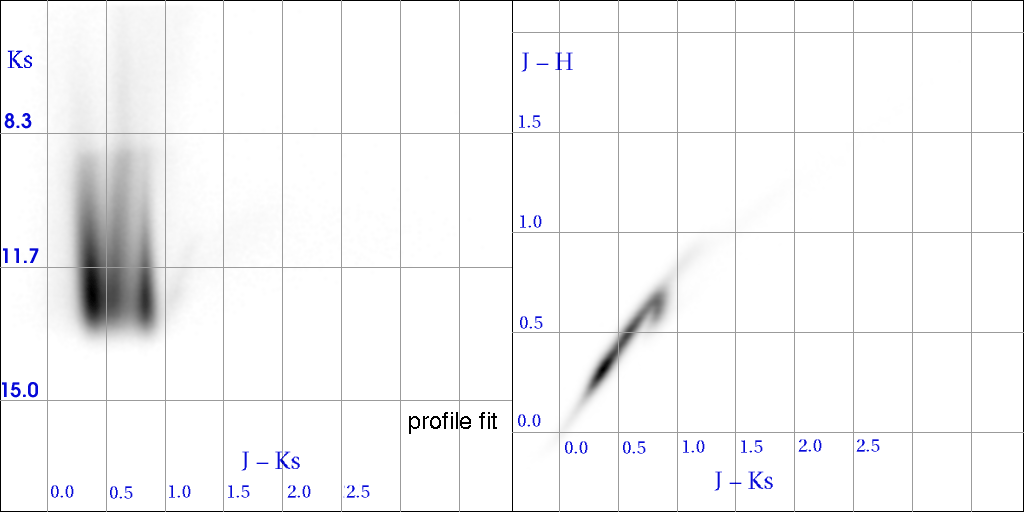
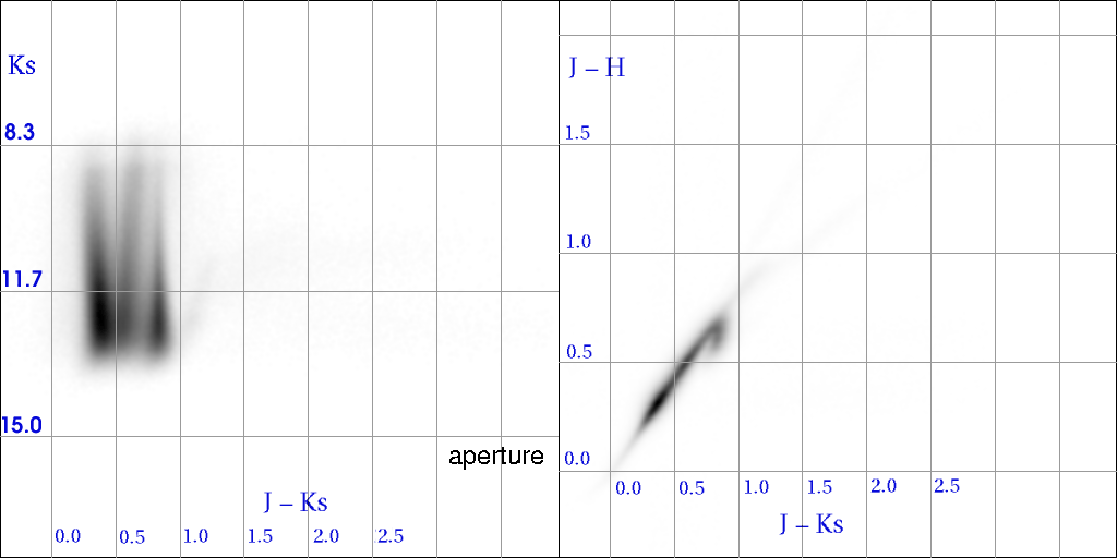
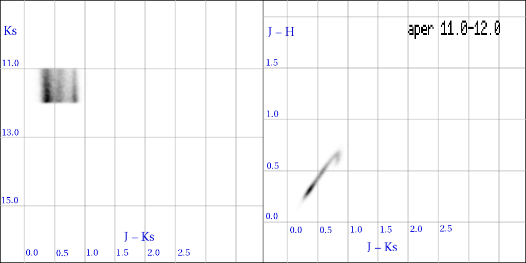
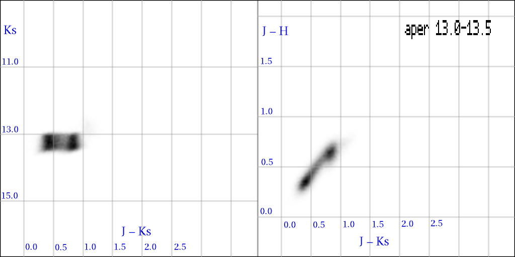
Aperture photometry provides the ultimate photometric precision for bright sources ([jhk]_m_aper < 13.0), since it does not depend on the perfect matching of a source's spatial profile with a pre-determined PSF. At faint magnitudes ([jhk]_m > 13.0), however, the reduced spatial footprint of a PSF profile fit yields a superior flux relative to an aperture measurement (which necessarily incorporates a large background area). Figure 38 presents aperture photometry for bright stars. The color-color relationship is more sharply defined, compared with Figure 37. Figures 39 and 40 make direct comparisons between aperture and profile-fit results in two narrow magnitude ranges. For 11.0<Ks(mag)<12.0, aperture photometry is superior to profile-fit photometry. For 13.0<Ks(mag)<13.5, the reverse is true.
Bright stars are absent in the color-magnitude diagram of stars with [jhk]_m_stdap aperture magnitudes in the PSC database (Figure 38). This column was populated with an aperture magnitude only if the source had a valid profile-fit detection (and thus only if the star did not saturate the 1.3 s exposure). Aperture photometry was used exclusively to produce rd_flg=1 photometry extracted from the 51 ms "Read_1" exposure; however, this value becomes the default magnitude, [jhk]_m, for the source and does not appear in the ( [jhk]_m_stdap) column. The [jhk]_m_stdap column is null for rd_flg=1 detections.
 |
 |
 |
| Figure 38 Aperture Photometry |
Figure 39 Blink Comparison with profile-fit 11.0<Ks<12.0 |
Figure 39 Blink Comparison with profile-fit 13.0<Ks<13.5 |
[Last Updated 2003 Oct 3; M. Skrutskie & J. Carpenter]
Return to Section II.2.