

C. Subtract darks from photometric checks and science scans:


NOTE: This document is subject to change due to ongoing IA/ISAP
software development.
To begin: Start your IA session by typing ia at the system prompt. Then follow the instructions below.
1) cal_select (help: IA UTILITIES)
This tool is used to select calibration files. See Appendix B.4 of the IA User's Manual for descriptions of each calibration file. The cal_select command opens a window which lists all current calibration files, and there are two possible settings for each CAL file: 'BASE' or 'TEST'. The 'BASE' system contains the CAL file configuration as in the current pipeline version. The 'TEST' system provides CAL files, which were updated since the last pipeline delivery. The individual choice depends on the current status of the CAL file system, so ask an IA guru. If you run the cal_select tool for the first time, save the recommended CAL file selection as file 'cal_select.dat' in your top directory. To do this, press the 'save' button after the CAL file selection, edit, if necessary, the 'path' box in the popping up window and confirm path and filename by clicking 'OK'.
If you have already saved the cal_select.dat file in a previous run of cal_select, you can restore the saved setting by clicking the 'load' button. NOTE: the 'path' box must be filled in properly, otherwise cal_select will crash.
After either setting (and saving) the appropriate CAL file selection manually or loading your calibration file, click 'OK' to exit the cal_select tool. All CAL files selected from the 'TEST' system are then listed in your test window.
2) erd=read_ferd('xxxYYYzz',path=[.data]) (help: IA INPUT OUTPUT)
This command reads in the ERD from the raw data files. The 8 digits in parentheses refer to the revolution number (xxx), target number (YYY), and observation sequence number (zz) from the archive listing. You may also use the command "read_fspd" to read in the SPD directly and skip to step 5; however, the pipeline reduction is ever-changing, and starting with the ERD you allows you take advantage of the most recent version of the reduction software and calibration files.
3) spd=dspd(erd) (help: IA DERIVE SPD)
This command converts the ERD to an SPD, using the following CAL files: (1; 2; 2a,b; 3; 4; 5; 6; 12; 16a,b,c,e; 18; 23; 24).
4) spd_orig=read_fspd('SWSPxxxYYYzz.FITS')  (help: IA INPUT OUTPUT)

		 spd.header=spd_orig.header
		 spd.data.det.flag=spd_orig.data.det.flag
		 save,spd,file='spd.save',/xdr
Unfortunately, the SPD header and detector flags (esp. the reference scan flag of SWS06) are not properly filled by dspd; the three commands in this step correct this problem by reading in the SPD (spd_orig) directly and copying its header and the detector flags into your recently derived SPD (spd). The filename given to read_fspd is in the format of files coming directly from the archive, where 'xxxYYYzz' are the same digits entered in step 2 above. The fourth command saves the SPD into an IDL save set, which can be restored in later sessions of IA if necessary.
In that case, typing
restore,'spd.save' (help: ROUTINES)
will restore the IDL structure spd to your IA session.
NOTE: An SPD is rather large, and the use of the option /xdr makes the saving process significantly faster. The /xdr (for eXternal Data Representation) option is not necessary to save smaller quantities such as the sctbl or aotlr alone (e.g., step 6), but it is needed if you wish to export any save sets between VMS and UNIX machines (see the IDL help file on "save" for more information.)
5) list_header,spd    (help: IA UTILITIES)

		 set_plot,'ps
		 device,file='aper_plot.ps',/landscape

		 aper_plot,spd,'1A',60.   (help: IA UTILITIES)

		 aper_plot,spd,'3A',60.
		 aper_plot,spd,'3E',60.
		 aper_plot,spd,'4',60.
		 device,/close
		 set_plot,'x
These tasks give you more information about your dataset. The list_header command lists the FITS header, and in particular, you should note the position angle INSTROLL of the y-axis of the ISO satellite during your observation (see ISO Observer's Manual for the definition of the ISO coordinate system). The position angle of the long side of the SWS aperture is then defined by: INSTROLL + 90 degrees.
The remaining commands in this step create a postscript file containing plots of the four SWS apertures on the sky (for bands 1 & 2; 3ACD; 3E; and 4). The value of 60. above is the declination scale of the plot in arcseconds. Consult your local system manager for printer options to determine how to print the postscript file locally.
6) sctbl=make_sctbl(spd) (help: IA UTILITIES)These commands create, print out, and save the scan table, which gives such information as the sequence of observations (darks, photometric checks, reference scans and science scans) and wavelengths covered by each scan.
print_sctbl,sctbl,file='sctbl.txt',/spawn
save,sctbl,file='sctbl.save'
The reference scans are specific for SWS06. They are short, pseudo-science scans, which were thought for additional calibration purposes, but never used in SWS06 reduction. Since summer 1997 they are no longer part of SWS06 observations. Usually reference scans are not passed into the AAR, unless the keyword /all is used in the 'daar' or 'extract_aar' command. Unfortunately, due to software problems, this keyword has currently to be used. The reference scans have therefore to be sorted out on AAR level. WARNING: for high fluxes, where memory effects play an important role, the continuum level of reference scans after dark measurements is too low. In combination with proper science scans they therefore might create fake features, if they would be included in the AAR.
The print_sctbl command prints the scan table to the screen as well as to the specified file name. The /spawn option is a local MPE command to print the specified text file to the default printer; again, consult your local system manager for printer options.
7) spd_mem=antimem(spd) (help: IA AUTO ANALYSIS)
This routine is designed for reducing memory effects, as is done in the standard pipeline. The use of antimem is mostly historical, but should be kept in the reduction chain because this task may in the future include a more complicated method for dealing with memory effects.
8) spd_D=dark_inter(spd,sctbl,/multia)  (help:IA UTILITIES)

		 save,spd_D,file='spd_D.save',/xdr
NOTE: Usually the server or window system is configured to retain plot window after scrolling or the start of a screen saver. The /multia option is only needed if the draw window is not retained (as on a Multia terminal); it causes IDL to handle the plot storage directly. The dark_inter tool facilitates dark current correction. It can be the most time-consuming of all data reduction steps, but is also one of the most important in producing reliable spectra. Make sure to save the SPD after completing this task. Before you begin, you should note the sequence of darks and other scans in the scan table. Note that the reset time ("tr") and gain columns in the scan table must be the same for a dark and the scan from which it is being subtracted; dark_inter automatically makes available all darks with matching tr and gain. Also check the scan table to determine which (band+scan) combinations hold actual data: those which do not will show "0.000" for both wave_min and wave_max (this information is also shown in the message box in dark_inter as "w_range"). It is not necessary to dark subtract these (band+scan) combinations. For each of the four bands (starting at detectors 1 [SW1:], 13 [SW2:], 25 [LW1:], and 37 [LW2:]), the following sequence should be followed:
A.Select a detector. This detector will represent the whole band.
B.Revise Darks. Click "Revise Darks". In the "Revise Darks" window which pops up:D. Set slider on top to the first detector number of the next band and repeat the process, starting with Step B, Revise Darks. Complete Steps B and C for all four bands. It is a good idea to save the data set periodically during the use of dark_inter, to prevent loss of efforts in the event that the tool crashes. The easiest way to do this is to use the "save current" button in the dark_inter tool, which creates a file called "dark_inter_save.xdr" containing the current data file. This file is overwritten in successive uses of this button, so you may make incremental saves without using additional disk space.

choose clipping options-here are the most general suggestions:


refine dark to be subtracted for each detector of the band, for each scan:


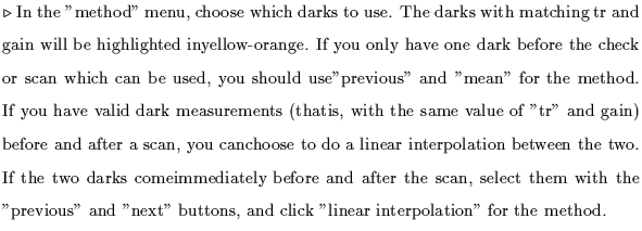
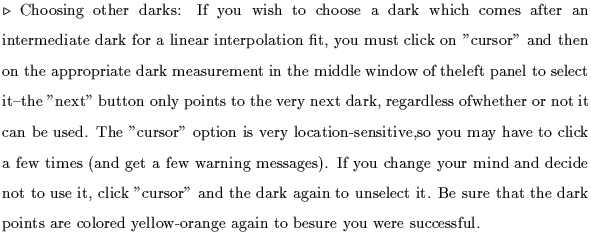
C. Subtract darks from photometric checks and science scans:

Choose the dark subtraction method: click on "Method".


Click "Done" in the Method menu.
Subtract fitted dark current.


9) spd_DM=mask_inter(spd_D,sctbl) (help: IA UTILITIES)This command puts you into the mask_inter tool, which can be used to inspect your SPD and mask out bad data. Sometimes a whole detector is significantly noisier than the others in the band, or there may be significant memory effects after a strong glitch. In addition, you can mask out the jump segments first detected with dark_inter (see step 8C). See the on-line help for this tool for a detailed account of all the utilities of this tool.
save,spd_DM,file='spd_DM.save',/xdr
Enter a band number in the "band" box, click on the scan number you wish to see, and click "disp_spd" to display a subset of the data. Note that to examine a different scan, you must click on the previous scan number again to "unset" it; otherwise there will be two scans selected and the tool will complain (multiple scans can be selected for producing an AAR within mask_inter, but only one scan can be displayed at a time). If you click the ``plotmode'' button, a background window will pop up in which you can set the plot scale; we recommend that you choose a fixed y-scale, as this is a good way of finding detectors for which dark subtraction didn't work properly, or for finding noisy detectors or other strange features. Each time you change the plot scale, click "disp_spd" again to display the data with the new plot values.
To mask out a specific section of a detector, click "select" and the detector of interest, which will cause the data from that detector to show in the bottom left window. Then click "mask" and use the left mouse button to select the region to be masked out (e.g., in the case of a memory effect). If you see the same glitch in all 12 detectors of a band, you can use the "do to all" button after masking out the glitch in one of the detectors. If you judge the input from an entire detector to be bad, you can click on the detector number in the list to the right-hand side of the display, and then click "faulty" to set it all bad.
IMPORTANT NOTE: Using the "faulty" button to set a detector "bad" is NOT reversible at the current time, and sets the specified detector bad for all scans. Setting the detector bad by masking all points out using the "mask" button IS reversible (using "unmask"), and only sets the detector bad for the specified scan.
Saving the masked SPD should be considered if a significant amount of masking has been done.
10) spd_U=aas_updowncal(spd_DM) (help: IA AUTO ANALYSIS)
Currently no interactive tool to correct for differences between SWS06 'up' and 'down' scans is available. Therefore the pipeline routine is used, which, due the lack of an proper automatic up-down calibration procedure, essentially does nothing to the data.
A patch is available for SWS02-like, short range scans with SWS06, of e.g. spectral lines, which were too broad for SWS02 line scans. Here an additional pseudo scan table sctbl_pseudo_S02.txt is created, which pretends the SWS06 DARK-UP-DOWN-DARK sequences to consist of SWS02 DARK-UPDOWN-DARK scans. Additionally a procedure file sctbl_6to2_patch.pro is created, which e.g. masks the data points inbetween the SWS06 UP-DOWN scans. A very careful inspection of the pseudo scan table and the procedure file is strongly recommended before use!
10') sctbl_pseudo_S02=make_sctbl(spd,undoc=2)       (help: IA UTILITIES)

		 print_sctbl,sctbl_pseudo_S02,file='        sctbl_pseudo_S02.txt'

		 @sctbl_pseudo_S02

		 spd_U=updown_inter(spd_DM, sctbl_pseudo_S02)       (help: IA UTILITIES)

		 save,spd_U,file='spd_U.save',/xdr
We refer the reader to the document 'Reducing AOT SWS02 Data in IA' for a description of the updown_inter routine.
11) plot_phot,spd_U,sctbl,[1],13,/all      (help: IA UTILITIES)

		 plot_phot,spd_U,sctbl,[1],25,/all

		 plot_phot,spd_U,sctbl,[1],37,/all
The routine plot_phot can be used to look at photometric check data. The command lines given above request IA to plot the first photometric check for all 12 detectors of bands 2, 3, and 4 (which start with detector numbers 13, 25, and 37); the band 1 photometric check is not used. If you have more than one photometric check, you can replace the [1] above with a range of values (e.g. [1,3]) and compare them on the same plot. By specifying a particular detector and removing the /all flag, you can look at the photometric checks for that detector.
Data points already flagged as bad by the system will be marked (see help file for color code). If these are the only bad points and the photometric checks look sensible, the standard routines will handle the bad points appropriately. Note that the default is to always use the first photometric check, so if it is corrupted it should be replaced with another. If you suspect your photometric data has problems which are severe enough to affect the ultimate calibration, such as a corrupted first photometric check or large spikes not already flagged, consult an IA guru.
12) spd_U=respcal(spd_U)      (help: IA AUTO ANALYSIS)

		 spd_U=fluxcon(spd_U)
		 spd_U=velcor(spd_U)
The routines respcal and fluxcon perform responsivity calibration and flux conversion and apply various calibration files; respcal uses CAL files 13, 19, and 25; fluxcon uses CAL file 13. The output of fluxcon looks like the following:
Warning(SPCP): some phot. check data might be doubtful       Det:26 Uv: 2
Warning(SPCP): some phot. check data might be doubtful       Det:39 Uv: 2
Warning(SPCP): some phot. check data might be doubtful       Det:46 Uv: 3
Warning(SPCP): some phot. check data might be doubtful       Det:48 Uv: 2
If the number following "Uv:" (i.e. the unvalid data points) is greater than 3, the photometric check data for that detector indicated may be suspect. The task velcor performs a correction to the heliocentric frame based on the velocity of the satellite. The velocity is taken from the SPD FITS header. 0.0 km/s are applied, if the SPD header is not properly filled (cf. step 4).
13) spd_F=flat_inter(spd_U,sctbl)  (help: IA UTILITIES)

		 save,spd_F,file='spd_F.save',/xdr
The first command starts up the flatfield correction tool flat_inter.
This task corrects the flatfield of each detector in the band with
respect to the others. As with "updown_inter", the correction can be
a "gain" or "offset" correction, and is made on the basis of smoothed
data. It is generally recommended to use the "median" filter, and to
exclude poor points. As with updown_inter, you should make sure that
the fit you have chosen does not introduce spurious features, and vary
the smoothing or correction parameters accordingly. The default
values are Res1=500 and Res2=100; try lower values, especially for
band 4 (LW2:) for very faint sources, and larger values may be useful
for very bright sources. In general, it is a good idea to keep the
relation Res1![]() 5 Res2. As before, the 'gain' option should only be
used with strong signal. NOTE: be sure to press "return" after
changing each entry; otherwise, strange effects may result if new
values are not registered by the tool.
5 Res2. As before, the 'gain' option should only be
used with strong signal. NOTE: be sure to press "return" after
changing each entry; otherwise, strange effects may result if new
values are not registered by the tool.
Faulty detectors might be specified with the faulty=[...] keyword, which contains the numbers of the bad detectors as a vector. These detectors are flatfielded anyhow, but not used for the definition of the flatfield itself.
14) spd_FM=mask_inter(spd_FM,sctbl) (help: IA UTILITIES)Now that all calibrations have been applied, you can go back into the interactive masking tool used in step 9 to mask out noise spikes or outliers; for instance, a signal which is clearly spurious, such as a strong spike detected only in the up or down scan of all 12 detectors, will bias the resulting spectrum. This masking step may be best done after following the rest of the steps described below and looking at an unmasked version of the output spectrum to see where lines have been detected, and returning to this step to produce a refined dataset.
save,spd_FM,file='spd_FM.save',/xdr
Click the "w-mode" button to plot in wavelength units, and specify the wavelength range of interest in the ``plotmode'' pop-up window. You can use the ``fluxclip'' button to mask out outlying data by hand. When you click this button, the data from all detectors is plotted in the lower left hand window, and you can define a series of boxes with the left mouse button; the points inside these boxes are then clipped. Clicking the right mouse button returns you to the main mask_inter tool. If you want to remove an unwanted glitch (glitches are marked with yellow asterisks), click "select" to specify the detector, and if needed click "zoom" and use the cursor to select the section of the scan holding the offending point (both up and down scans will be shown, with wavelength units along the upper x axis of the plot). Then click "unglitch", and click the mouse cursor on either side of the glitched point. The unglitched point will show up as a white cross, like the rest of the good data.
You can see the effects of your masking by using the "extract_aar" and "aar_f" buttons, which will produce a filtered AAR (with the resolution specified in the "resol" window) of the specific section of spectrum that you have selected with band, scan, and x_range. It is recommended to use kappa=2.5-3 and resol>2000, especially for faint sources. Further, you can output your final, masked AAR result to a file by clicking on the "save_aar" button. This action will pop up a window where you can specify the name of the file you wish to write, and what format: XDR, IDL SAVE, or FITS. The first two options both write IDL save files which can be restored in an IA session (the first using the XDR format described in step 4). Repeat for each line.
15) spd_FM=killwait(spd_FM)  (help: IA UTILITIES)

		 aar=extract_aar(spd_FM,/all)     (help: IA AUTO ANALYSIS)
		 save,aar,file='aar.save',/xdr
		 status=sap_wfits('aar.fits',aar)  (help: ISAP)

		 range=aarfilt(aar,[6.92,7.32],1200.,kappa=3.0,/noglitch)
The first task flags "wait" points as "bad"; it is useful on SWS01, SWS02, and
SWS06 data. The next task extracts an AAR from the reduced SPD. The keyword
/all, which has to be used due to current software problems, makes sure that
all scans, including the reference scans are passed to the AAR (cf. step 6).
The following two commands save the AAR as an IDL save set and a FITS file.
Note that all the masked and glitched points are still in the AAR, but are
ignored in aarfilt on request by keyword /noglitch.
The last task produces a final, filtered AAR for a particular SWS06
scan; you should repeat this step for each individual range. In
this example, the wavelength range is 6.92-7.32 microns, the
resolution is 1200, and kappa is set to 3 (3![]() ). Save the
individual filtered files as the whole AAR was saved above. If you
have faulty detectors that were not masked out before, you can do so
with this command as well-see the help file.
). Save the
individual filtered files as the whole AAR was saved above. If you
have faulty detectors that were not masked out before, you can do so
with this command as well-see the help file.
After this step, the basic reduction of SWS06 data is complete, but there is likely significant fringing, especially for lines lying in bands 2 and 3. These can be good to deal with for SWS06 data, if they cover a long baseline containing many fringes. There are different tools you can use to defringe, either by trying to remove the fringes or fitting a line shape; these include linefit (in ISAP), aarfringe, or multifit. Consult your IA guru for strategies for recovering as much information as possible.
Finishing up:
Type ``help'' to look at the list of IDL structures you have generated in this data reduction section. Make sure to save all files which were produced from the most time-consuming steps (i.e., any of the interactive tools) as IDL save sets and FITS files before exiting from IA. Then you can restore the SPD or AAR at any stage and redo some of the reduction if you find it necessary at a later date.