The ability to separate real extended sources (e.g., galaxies, nebulae, H II regions, etc) from stars is what fundamentally limits the reliability of any extended source catalog. Single isolated point sources represent the purest construct at which extended sources are compared and separated. More complicated constructs include ædoubleÆ stars and ætriple+Æ stars. The ædoubleÆ and ætripleÆ monikers are generic labels that include physical multiple systems and, more likely, chance superposition of stars on the sky. There are endless permutations and combinations of multiple-star characteristics (radial separation, flux difference, color difference, etc) which provide a thorny challenge toward separation from real galaxies. What is more, for 2MASS and most other all surveys, stars greatly outnumber extended sources by a ratio of something like ~10:1 in most of the sky (near the galactic plane the ratio is yet orders of magnitude larger), so for every resolved galaxy in the sky there are plenty of double+ stars camouflaged as extended sources. The art of separating stars from galaxies is generally at a mature state in the field of astronomy with many competing methods that are for the most part very effective at their job. From the simplest "CART" methods (i.e., linearly measuring one attribute versus another) to the more sophisticated Bayesian-based methods (e.g., FOCAS; see Valdes 1982), decision trees (cf. Weir, Fayyad & Djorgovski, 1995) and neural networks (cf. Odewahn et al, 1992), each designed in response to increasingly more complicated data sets. For 2MASS, we were faced with the rather unique combination of near-infrared imaging and under-sampled data (2" pixels with a PSF that is quasi-stable) that called for yet a new approach at star-galaxy discrimination to satisfy the rigorous level-1 specifications. Early experimentation with tried and true algorithms (e.g., FOCAS) were unsatisfactory primarily due to the severely undersampled 2MASS PSF that changes width (and symmetry) over real times scales of minutes. Accordingly, the bulk of the 2MASS extended source processor, GALWORKS, is dedicated to the multi-layered task of star-galaxy separation. The basic approach is for GALWORKS to accurately measure and track the time-varying PSF and compare it with several different object attributes (i.e., parameterization) by applying some simple CART-like rules to cull out most of the multiple stars and other non-galaxies that mimic real extended sources. The resultant extended source database is approximately 80% reliable for most of the sky. In a post-processing phase, further refinements, including more complicated attribute combinations and decisions trees, are used to produce the extended source catalog at a reliability of greater than 98% for K < 13.5. Below we describe and discuss some of the more critical parametric measurements and decision tree operations to that end.

Resolved sources are identified as such by comparing their radial profiles with that of the nominal point spread function. As is the case for all ground based observations, the PSF changes with time due to the changing thermal environment and dynamic atmospheric "seeing" (see section 2.4), and additionally, the PSF has an intrinsic spread caused by the pixel undersampling and dither pattern. Both affects are measured and tracked using our generalized exponential function (section 2, Eq. 1) and stellar ridge profiles (e.g., section 2, Fig.??). The radial "shape" (a ´ b), or simply "sh", of a source is compared to the stellar ridge value, sh₀, and a N-sigma "score" is computed thusly,

where sh₀(tÆ) and Dsh₀(tÆ) denote the time variable ridgeline value and its associated uncertainty and sh(t) the source value, with time tÆ as close to real t as possible. The PSF ridgeline value is stable over all flux levels, so only one value is needed per time interval. The "sh" uncertainty folds in both measurement error and the intrinsic PSF spread. However, since SNR > 10 stars are generally plentiful, the measurement error is for the most part minimal compared to the real spread in the PSF. The uncertainty represents the RMS in the "sh" distribution and is used analogously to a gaussian dispersion, but we note that the distribution is not gaussian shaped in reality, instead it has triangular-shaped wings (i.e., the scatter in "sh" falls of linearly). Consequently, stars will not have "sh" values above a threshold of ~2*Dsh₀, but galaxies and other relatively æextendedÆ objects (e.g., double stars) will have scores >2. In Figure 1 we illustrate with the J-band "shape" score (Eq. 2) three kinds of objects that 2MASS is likely to encounter, in order of numerical importance: stars, multiple stars (double stars and triple+ stars), and galaxies. Stars occupy a locus about zero "sh" score (essentially defining the ridgeline), while multiple stars lie well above the ridgeline along with galaxies and other "fuzzy" sources. The "sh" score is very effective at separating isolated stars from galaxies at flux levels as faint as ~15.4 in J band.

Other GALWORKS-derived image parameters that are effective at separating isolated stars from galaxies include the 1^st and 2^nd intensity-weighted moments, ratio of the central surface brightness to the integrated brightness, and areal measures (e.g., isophotal area).

Unfortunately, like the radial "sh" parameter, all of these diagnostics are ineffective at separating galaxies from sky-projected star clusters. Double stars are in particular a vexing component due to their sheer numbers at galactic latitudes < 20° . Figure 2 shows the expected number of double stars and triple stars as a function of galactic latitude (with longitude fixed at 90° ) for K (system) < 13.5. Sky-projected doubles contribute ~2% of the total at high glat, but quickly begin to dominate the total numbers for latitudes less than 5 degrees. Even at low stellar number density, double stars still outnumber galaxies in number density for typical 2MASS flux levels. We clearly see that double stars (and triple+ stars near the galactic plane) are the primary contaminant of the galaxy database. More intricate attributes are needed to exploit the differences between groupings of point sources and real fuzzy objects (resolved galaxies).

In the near-infrared galaxies consistently exhibit the morphological feature of smooth radial and azimuthal profiles. Their æsymmetricÆ near-infrared light distribution is the composite outcome of photospheric emission from the older stellar populations, including low mass dwarfs (e.g., G & K dwarfs) and intrinsically bright evolved stars (e.g., K giants), generally spread evenly throughout the disk and bulge regions (spirals). Large-scale features commonly seen in the radio and optical wavelengths, including H II regions, supernovae remnants, disk warps, and dust lanes, are generally lacking in the near-infrared except for the largest (nearby large angular diameter) galaxies. Only the relatively rare cases of galaxies subject to tidal or hydrodynamical interaction exhibit significant asymmetry in the near-infrared bands. In contrast, multiple stars, and in particular double stars, are not symmetric about their æprimaryÆ center. Here the center of a multiple star corresponds to the brightest member in the group, or more specifically, the peak pixel associated with the primary (again, we are, for the most part, referring to chance superposition of stars on the sky). The near-infrared symmetry of galaxies can be exploited to differentiate between multiple stars that otherwise mimic extended sources.

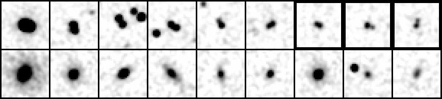
Figure 3 illustrates some of the kinds of double stars seen in 2MASS images. For comparison, a set of galaxies of approximately the same integrated brightness as that of the double stars is also shown. For double stars, the æsecondaryÆ component of the system is what breaks the symmetry of the primary, which otherwise would have the symmetric shape of the PSF. One of the obvious symmetry attributes is to ratio the integrated flux as measured on one side of the primary and on the opposite side (containing the secondary star). The system is defined as an ellipse with the primary at the center and the secondary along the major axis.

A different tact is to æremoveÆ the secondary and measure the resultant "sh" of the primary. We are of course faced with the problematic fact that the emission from both sources are entangled and the primary itself has changed both its radial ("sh") width and its azimuthal (symmetry) shape. If the PSFs were exceptionally stable and well characterized as such, then in principle it would be possible to satisfactorily de-blend the multiple sources into their constituent parts. Since this condition is never realized, and moreover the runtime for this kind of PSF c ² fitting is prohibitively long, we are left with the only option of bluntly removing the secondary. The æblindÆ approach is to remove the secondary using a median filter in annular shells about the primary (GALWORKS refers to the resultant measure as the "median shape" or just "msh"). The direct approach is to mask the secondary and measure the residual primary. We have developed a direct approach that uses a wedge or pie-shaped mask that is rotated about the vertex-anchored primary. The optimum configuration in which the secondary is effectively masked is found by rotating the wedge mask through all angles (see illustration below).

The "sh" score (Eq. 2) is then computed for the remaining (360° û 45° ) pixels. If the secondary star is masked, then the resultant "sh" score will be minimized, ideally with a value corresponding to an isolated star. In practice the secondary can never be fully masked, and the peak pixel does not represent the true center of the primary since it is slightly shifted toward the secondary û thus resulting in an artificially inflated "sh" score relative that of an isolated star. Nevertheless, the "wedge" shape score, or simply "wsh", turns out to be an effective discriminant, as demonstrated in Figure 4. Analogous to Figure 1, here we show the distribution of multiple stars and galaxies as measured in the "wsh" versus magnitude plane.

The wedge shape score for double stars is considerably smaller than the corresponding "sh" score, having values typically less than 5 for J < 15, while galaxies remain "extended" in this measure with scores >5 for J < 15. Note however, triples+ stars are only minimally affected by the "wsh" score since by definition they have at least two secondary components which in the end defeats the single rotating mask method. For triple stars, yet more severe "symmetry" constraints are required.

Triple stars are geometrically more difficult to characterize due to the added complexity of an additional component (thus more possible combination of the integrated flux and the primary-secondary separations). The æAchilles' heelÆ of triple stars, however, is that along some vector (anchored to the primary) there is minimal contamination from the two secondary components. If we measure the radial "sh" of this vector and compare it to the corresponding ridgeline value, the resultant æscoreÆ should be close to that of an isolated star. Thus the basic method is to measure the "sh" along an azimuthally distributed set of vectors (angular separation 5 deg). Departures from this ideal solution are the usual culprits: contamination from the secondary(s) shift the primary peak pixel and drive flux into the radial/azimuthal profile of the primary. The vector corresponding to the æminimumÆ shape score (referred to as the "R1" score) is susceptible to background noise fluctuations since we are restricting the (a,b) fitting operation to less than a dozen pixels. For galaxies, the "r1" score tends to select against galaxies that are edge-on and thus have minimal (but still measurable) extended emission along the minor axis (i.e., the vector corresponding to the minimum radial "sh" score). A more robust parameter (but slightly less effective at removing the influence of the secondary components) is to average the 2^nd and 3^rd lowest "sh" value vectors (that is, avoid the "r1" vector). This score is referred to as the "r23" shape score. Here we are relying upon the fact that most triple star configurations (but not all by any means) will have more than one vector that is minimally affected by the secondary components. Galaxies, meanwhile, are generally extended in all directions and so the "r23" score is not much different from the "sh" score except for the faintest galaxies (J > 15, K > 13.75) which are at the mercy of noise fluctuations. The effectiveness of the "r23" score is demonstrated in Figure 5. Here we plot the "r23" versus magnitude phase space. It can be seen that the triple stars are now well under control with minimal loss to the galaxies at J < 14, while for the faint mag bins, J > 14, galaxies are not well separated from triple stars. But, as it turns out, triple stars are only abundant when the stellar number density is very high (i.e., the galactic plane; see Fig 2), which means that the æconfusionÆ noise is also high (that is, the random fluctuations in the background due to faint stars) , rendering the sensitivity limits for galaxy detection itself from 0.5 to nearly 2 mags brighter than the nominal 2MASS limits. Thus, just as the problem with triple stars becomes significant, the detection thresholds are correspondingly decreased, thereby leaving the "r23" score as an effective star-galaxy discriminator for flux levels up to the detection limits. For the most extreme stellar number density cases (e.g., regions of BaadeÆs windows), >10⁵ stars per deg² brighter than 14^th at K, quadruple ++ stars become significant, at which point there is no way to separate galaxies from clusters of stars.

We have developed additional parameters designed to minimized contamination from triple stars, including flux gradients along radial vectors (referred to as the "vgrad" score) and integrated flux along radial æcolumnÆ vectors (referred to as the "vint" score). Similar to the "r1" and "r23" scores, these methods rely upon the æminimumÆ column integrated flux or gradient in the column flux to be similar to that of isolated stars. They are not quite as effective as the "sh" vector scores, but since they are only slightly correlated, they can be used in combination with the other attributes to using a decision tree.

For similar reasons that galaxies appear smooth and symmetric in the near-infrared (section 4.2), they also display consistently redder colors relative to typical field stars. Two effects conspire to make galaxies "red" in the 1-2 mm window: their light is dominated by older and redder stellar populations (e.g., K and M giants), and their redshift tends to transfer additional stellar light into the 2mm window (for z < 0.5). The latter phenomenon is rectified with what is known as a "K correction", or a model-dependent flux correction to the observed colors. In view of that, the J-K color attribute can be used û in conjunction with color-independent discriminants, like the "wsh" score -- to cleanly separate extragalactic objects from stars. As a bonus, the color separation is enhanced in the galactic plane where double and triple star contamination is severe. Since galaxies lie behind the obscuring disk of the Milky Way, they are subject to a larger column density of gas and density compared to random field stars along the same line of sight and thus are redder due to selective extinction. We demonstrate the effectiveness of the J-K color to separate stars from resolved galaxies in a diverse set of fields, including areas well above the galactic plane, referred to as low stellar density fields (<10^3.1 stars per deg² brighter than 14^th at K), and areas closer to the plane (glat > 5 degrees) , referred to as moderate density fields ( <10^3.6 stars per deg²), and finally areas in the galactic plane in which the stellar number density is very high (>10^3.6 stars per deg² brighter than 14^th at K). For the latter case, the confusion noise is typically very high (>1 mag) so the sensitivity limits have been decreased accordingly.

The J-K color for galaxies and double stars located in low density areas is shown in Figure 6. Here we ignore the contribution of triple stars to the total mix (since their numbers are insignificant in these areas). Figures 7 shows the color distribution for sources located in moderate density fields, and Figure 8 sources from high density fields.

A J-K color of 1.0 appears to be a natural border separating stars from galaxies. For flux levels relevant to the 2MASS level-specifications, K < 13.5, a J-K color limit of 1.0 eliminates nearly all (>95%) double stars that mimic galaxies, while more than 90% of the total galaxy distribution has a color greater than this limit. The same trend is observed in the more confused regions of the sky (Figure 7 & 8) where star-galaxy discrimination is at a premium. Another way to view the color separation between stars and galaxies is within the J-H vs. H-K color plane, Figures 9,10,11. Here we include the stellar main sequence track, showing the divergence of giants from dwarfs at H-K > 0.3. In addition, we note the K-correction track for spiral galaxies derived from the models of Bruzual & Charlot (1993).

At fainter flux levels, K > 13.5, the scatter in the integrated flux (and thus colors) is large enough that false galaxies (i.e., double and triple stars) can scatter above the J-K color limit and galaxies can have colors that scatter below the limit to a degree that contamination and completeness is compromised if the J-K attribute were used as the lone discriminant. Moreover, for all flux levels, a J-K threshold would impart an undesirable selection bias against blue galaxies. To minimize color biases, the J-K attribute can be combined with the radial shape attributes (e.g., the "wsh" score) to form a new powerful discriminant. First, the color-color plots suggest a better method to use JHK colors to measure the "redness" of a galaxy. Galaxies are not only preferentially redder than 0.9 in J-K, but they also have H-K values, >0.2, redder than most stars. Consequently, we define the following "color score" as:

Color score = [(J-K) û 0.9] + {[ (H-K)>0.3] ´ [(H-K)-0.3]}

which adds the color ædistanceÆ from the dotted line in Figure 9. For sources with (H-K)>0.3, the color score reduces to:

Color score [(H-K) > 0.3 = (J-K) + (H-K) û 1.2

The color score can be directly combined with one of the color-independent attributes (e.g., "wsh") to provide additional star-galaxy separation. Figure 12 demonstrates the combination of color score and "wsh". This combination parameter alone is capable of providing better than 95% reliability (K < 13.5) with only a few % loss of galaxies to the total population. We can do better still by using all of the attributes with a decision tree.

Three classes of attributes have been introduced thus far: radial extent or shape ("sh", "r1", "r23"), symmetry or azimuthal shape ("wsh", "msh", flux ratio) and flux or photo-metrics ("vint", "color score", total flux, and central surface brightness relative to the total flux). We have something like a ninth dimensional space to probe (per band) for any given source to decide if it is extended. To complicate matters, several of the attributes are highly correlated (e.g., "wsh" and "msh") and others weakly correlated (e.g., "wsh" and the bi-symmetric flux ratio), which ultimately prevents simple or weighted combination of the attributes to form a "super" attribute. We may either combine a few of the attributes that are not correlated (e.g., color score and "wsh" and "r23"), see Figure 12, or employ a decision tree induction method (cf. Breiman et al. 1984) to effectively combine all of the attributes. In the last few years, decision trees and their close cousins, machine-learning artificial neural networks, have been used by astronomers to aide in image classification (e.g., Weir et al, 1995; Odewahn et al. 1992; White 199?; Salzberg et al. 1995). With fast computer technology these methods provide an efficient means to analyze multi-dimensional data. We will consider one particular type of decision tree, called the oblique-axis decision tree, but there are many others that should be effective. Neural nets also have been shown to be very useful for classification, but given their complexity and non-intuitive nature, we will not consider them at this time.

Decision tree methods, like artificial "neural networks", require a ætrainingÆ set of pre-classified (reliable) data composed of all combinations of stars (isolated, double, triple, etc) and galaxies. This "truth" set is used to generate the decision tree, or a structured set of classification rules. Using the analogy of a tree, the rule structure contains ænodesÆ of branching test points with the final nodes in the tree representing the æleavesÆ or final classification. For example, one node might represent a test of the "wsh" score, comparing the score to some threshold, T,

"wsh" score > T ?

NO: classify as non-galaxy

YES: continue to next node

This is an example of an "axis-parallel" decision. That is to say, the parameter or object attribute is embodies a set of hyperplanes (re: multi-dimension phase space) that are parallel to each other. Figure 13 demonstrates a two-featured, hyperplane: "wsh" score vs. J mag. The features correspond to what is relevant to the 2MASS project: galaxies (denoted by filled circles) and non-galaxies (crosses). The non-galaxies are mostly double stars in this example. The dashed parallel lines represent the axis-parallel "rules". To the right (or above) of the lines are the galaxies, to the left (or below0 the lines are the false galaxies or non-galaxies. Axis-parallel rules have the advantage of being simple to apply and track within a large complicated tree. But it is obvious from the example plot that a better rule is to use an "oblique" line separating the two populations or features. The solid line in Figure 13 is an example of an oblique-axis ruling. An oblique decision tree uses both axis-parallel and oblique-axis tests at the nodes. Mathematically, the node test has the form:

where object O possesses n attributes, with a coefficients or weights defining the n-dimensional hyperplane. For the reduced axis-parallel case, the linear sum reduces to a_jO_j > T. Although oblique hyperplanes are just a series of linear combinations, the total possible number of solutions is very high and thus finding the æcorrectÆ is daunting, if not impossible under all conditions. In fact, the problem is NP-Complete, or ultimately limited by the runtime of the machine. Fortunately, in practice reasonable decision trees can be generated with clever deduction algorithms and techniques to avoid "traps" or local minimum solutions. One such package was developed by Murthy et al. (1994) called OC1, or Oblique Classifier 1. OC1 uses random perturbations to walk around traps and arrive at proper (or more likely, satisfactory) hyperplane solutions for each node. The resultant tree may require æpruningÆ or stripping of branches that add little to the final classification, or worse, detract from the correct solution due to over-fitting of the training set (which is ultimately finite and limited). OC1 applies pruning methods, e.g., Cost Complexity pruning (cf. Breiman et al 1984), which effectively prunes the decision tree by removing the insignificant or "weak" branches. For the problem of over-fitting, in addition to pruning, the best solution is to minimize the total number of attributes per node. For 2MASS galaxies, nine attributes including the integrated flux characterize each source. The attributes are correlated to one degree or another, so it is not obvious which attribute(s) can be eliminated from the decision tree process. Experimentation with the training sets and additional pre-classified data sets give us the only clue as to the level of pruning that our decision tree requires. One disadvantage that decision trees have with classification of galaxies is that the final classification does not have an associated uncertainty or probability of being a galaxy. A probability is what is really needed, so the designers of decision tree algorithms have made this one of their priorities for future design. For 2MASS galaxies, we can "assign" a probability by using a weighted average of the decision tree classifications for each band (details given below).

The 2MASS star-galaxy separation problem is ideally suited to an oblique decision tree technique. Accordingly, we have applied the OC1 technique to large data (training) sets of 2MASS extended sources and non-galaxies (stars, double stars, triples, etc). The sets are delineated into three subsets, one for low stellar density fields, <10^3.1 stars per deg² brighter than 14^th at K, one for density fields, 10^3.1 to 10^3.6 stars per deg², and one for high density fields,>10^3.6 stars per deg² brighter than 14^th at K. The subsets are further divided into three or four sub-subsets depending in the integrated flux of the source. The latter step minimizes the severe dynamic range (in flux) that 2MASS must consider, from the brightest galaxies (K < 9) to the faintest galaxies (K > 14). The training sets are large and diverse (e.g., the low-density sets contains over 15000 objects, comprising some 280 sq. degrees) and thus provide a suitable induction test bed for the decision tree algorithm. Preliminary results show that with the OC1 decision tree classifier the galaxy catalog reliability increases several % compared to just using simple CART or axis-parallel tests. The trend persists in regions of high stellar number density where double and triple stars become a major contaminant. More detailed results of the completeness and reliability are given in section ??. Future work to refine the decision trees will focus upon further pruning of the trees and upon possible elimination of "weak" attributes. It may also prove fruitful to evaluate other decision tree methods (for example those developed by Weir et al. 1995; Fayyad 1994) and, possibly, artificial neural network methods, particularly if morphological classification is attempted (i.e., construing the galaxy type and sub-types) with 2MASS imaging data.

Figure 1-- Distribution of stars, multiple stars and galaxies in the J-band "sh" versus magnitude parameter plane. The sources do not come from the same sample; e.g., the triple stars are derived from high stellar source density fields in the galactic plane. Stars generally outnumber galaxies by a ratio of 10:1 for J brighter than 15^th mag.

Figure 2-- The expected fractional percentage (of the total) of doubles stars (triangles) and triple stars (crosses) with galactic latitude. The longitude is fixed at 90 degrees. The calculations are based on the starcount models of Jarrett (1992). Double stars, dominated by sky-projected associations, represent æprimary-secondaryÆ separations of less than 6 arcsec (the 2MASS PSF for comparison has a FWHM > 2 arcsec).

Figure 3--Examples of 2MASS double stars and galaxies. The upper panels demonstrate various kinds of doubles encountered. The lower panels show galaxies with approximately the same flux as their double star counterparts (left most panel: J = 11th mag; right-most panel, J = 15^th mag).

Figure 4-- Distribution of multiple stars and galaxies in the J-band "wsh" score versus magnitude parameter plane. The sources do not come from the same sample; e.g., the triple stars are derived from high stellar source density fields in the galactic plane

Figure 5-- Distribution of multiple stars and galaxies in the J-band "r23" score versus magnitude parameter plane. The sources do not come from the same sample; e.g., the triple stars are derived from high stellar source density fields in the galactic plane.

Figure 6ùHistogram of the J-K color distribution for galaxies and double stars. The upper panel is restricted to sources with K < 13.5. The middle panel represents sources at the sensitivity limit of the survey (K < 13.75) and the last panel shows sources generally fainter than the Kûband sensitivity limits (K > 13.75) but detected and extracted due in part to the superior sensitivity limit at J band. The data come from a diverse set of low stellar number density fields, comprising some 250 square degrees.

Figure 7-- Histogram of the J-K color distribution for galaxies and double stars in moderate stellar number density fields (10^3.1 û 10^.3.6 stars/deg²). The upper panel is restricted to sources with K < 13.5, and the bottom panel K > 13.75. The data come from a diverse set of moderate stellar number density fields, comprising some 150 square degrees.

Figure 8-- Histogram of the J-K color distribution for galaxies and double stars in high stellar number density fields (>10^.3.6 stars/deg²). The upper panel is restricted to sources with K < 13.0, and the bottom panel K > 13.0. The data come from a diverse set fields, comprising some 60 square degrees.

Figure 9--J-H vs. H-K color plane distribution for sources, K < 13.5, located in low stellar number density fields. Triangles denote double stars, crosses triple stars, and small points galaxies. The solid line demarks the main sequence tracks (dwarfs lower track, giants upper track). The K-correction track for spirals is shown with the dashed line. The large diamond symbols denote intervals of 0.1 in redshift (z).

Figure 10-- J-H vs. H-K color plane distribution for sources, K < 13.5, located in moderate stellar number density fields. Triangles denote double stars, crosses triple stars, and small points galaxies. The solid line demarks the main sequence tracks (dwarfs lower track, giants upper track). The K-correction track for spirals is shown with the dashed line. The large diamond symbols denote intervals of 0.1 in redshift (z).

Figure 11-- J-H vs. H-K color plane distribution for sources, K < 13.0, located in high stellar number density fields. Triangles denote double stars, crosses triple stars, and small points galaxies. The solid line demarks the main sequence tracks (dwarfs lower track, giants upper track). The K-correction track for spirals is shown with the dashed line. The large diamond symbols denote intervals of 0.1 in redshift (z).

Figure 12--Distribution of stars and galaxies in the "color score + wsh" space. The upper panel corresponds to low stellar number density; middle panel to moderate stellar number density; lower panel to high stellar number density.

Figure 13--An example of a two-featured data hyperplane set that is addressed within a decision tree node. A subsection of the "wsh" score û J magnitude plane for galaxies (denoted with filled circles0 and non-galaxies (denoted with cross symbols) is shown (derived from sample shown in Figure 4). Axis-parallel planes are represented with dashed lines and the best-fit oblique plane in represented with a solid line.