III. 2MASS Details

3. Data Processing

c. Point Source Detection and Photometry

As described in the introduction to section III.3, the detection and measurement of point sources is done several times during the processing of a 2MASS scan. Each detection and measurement step serves a different purpose. Sources are first detected and aperture-photometered from the individual dark-subtracted, flattened and sky-offset corrected R1 and R2-R1 frames. These detections provide positions to tie the frames together for Atlas Image generation (cf. III.3.b), and photometry for objects that are saturated in the R2-R1 (1.3 sec) exposures. Source detection is done on coadded Atlas Images for maximum sensitivity. Both profile-fit and aperture photometry is carried out for these fainter detections, although the measurements are actually carried out on the individual R2-R1 data frames to avoid flux biases caused by masked or aberrant pixels. The entries for each object in the 2MASS Point Source Catalog contain a "default magnitude" field for each of the three survey bands (j_m, h_m and k_m). These values represent what are believed to be the best estimate of a source's brightness in each band. The origin of those magnitudes is described in the "rd_flg" parameter, so users are urged to consult that flag for all objects. The subsections below describe each of the detection and photometry algorithms in more detail.

Frame Source Detection and Aperture Photometry

Point sources are detected in each instrumentally-corrected R1 and R2-R1 frame by identifying local intensity maxima. Positions are measured for these detections using a maximum-likelihood estimator, and magnitudes are estimated using aperture photometry within a 4´´ (two camera pixel) radius aperture.

The values for all the pixels are histogrammed, and the median sky value and the noise are estimated. The noise is estimated as one-half the distance between the 0.1587 and 0.8413 percentile points.

All the pixels in the frame are examined to identify local maxima. For each local maximum exceeding the local background by more than T_pk (where T_pk=4), the following computations are performed:

The centroid of the 3×3 patch centered on the local maximum is first evaluated:

(Eq. III.3.c.1)

(Eq. III.3.c.2)

(Eq. III.3.c.3)

The local centroid is used as the initial source position, which is then refined using the following maximum likelihood position estimation technique, with the cost function on each axis computed by:

	(Eq. III.3.c.4)

	(Eq. III.3.c.5)

P = the normalized point spread function (PSF) and F_t is the template amplitude,

(Eq. III.3.c.6)

C_x and C_y are followed to their zero crossings, and then interpolated to solve for (x_c,y_c).

The fraction of flux in the peak pixel (f_peak) is computed by:

(Eq. III.3.c.7)

• F_t / F_ap > T_frat (0.8)

• estimated source position is within r_pk (0.3) of the center of the pixel

• R2-R1 is being processed.

The aperture photometry module is called to compute the aperture magnitude at the estimated position.  The aperture photometry on a frame is performed by summing pixels entirely within the aperture and interpolating pixels partially within the aperture. The sky background for each object is computed in an annulus with an inner radius of 24.0´´ and an outer radius of 30.0´´. Pixels in the sky annulus are entirely included or excluded based on the distance of their centers from the source. The sky value is estimated by first excluding saturated, masked, or unreasonably low pixels. A sigma-trimmed median of the surviving sky pixels is then used as the sky estimate. Aperture photometry and positions from the maximum six possible overlapping frames are later combined using an unweighted average for the R1 data.

The 3×3 pixel patch centered on the peak pixel along with the coordinates of the peak pixel and the aperture magnitude and associated error are written to a temporary file so that the detection parameters may be re-estimated in a second pass using a PSF matched to the seeing.

Then:

• The f_peak histogram is interpolated for the 80th percentile value, which is written to a file, and used to redefine the PSF for the scan.

• The R2-R1 and R1 source patch files are reprocessed and the template amplitude, F_t, and the other parameters for each detection are estimated using the redefined PSF. The parameters for all extractions are written to files for R2-R1 and R1.

READ1 Aperture Photometry

The photometric dynamic range of 2MASS is extended by the use of the 51 ms R1 exposures. Sources saturate on the 1.3 sec R2-R1 exposures at magnitude levels of approximately 8.0, 7.5 and 7.0 at J, H, and K_s, respectively. For objects that are found to have one or more saturated pixels within the measurement aperture on the R2-R1 frames, the "default magnitude" quoted in the Point Source Catalog records is taken from the aperture photometry from the R1 frames. This is indicated by a value of "1" in the "rd_flg" parameter in the point source records, for the appropriate bands. Positions measured from the R1 frames are used in the final source position estimation only if R2-R1 profile fit results are not available.

The aperture photometry measured in this step for non-saturated R2-R1 sources from individual frames is not carried forward as part of the final source characteristics.

Faint Source Detection

The fainter, and thus majority of sources found by 2MASS are detected from the Atlas Images. Each Atlas Image is convolved with a zero-sum 4´´ FWHM Gaussian over a 13-pixel sub-array. The resulting zero-sum filtered image is thresholded, and for each maximum over threshold, a detection is identified and a rough position estimate is computed from the corrected centroid. This detection process is in all essential aspects identical to that used in the FIND subprocess of the DAOPHOT II program developed by Peter Stetson (P.B. Stetson 1991). The detections list is sent to the software module that computes the running estimate of the seeing during a scan, and to the photometry routines that compute the refined estimates of flux and position. The detection threshold used is 3.0 times the estimated noise level for the Atlas Image. The noise level is estimated as the difference between the 50% and the 15.87% quantiles of the image histogram. This noise estimator has been found to be excessively sensitive to low frequency noise due to airglow (OH), and will be replaced by an estimate computed from the zero-sum filtered image for the final processing of the 2MASS data.

Profile-Fit Photometry

The primary photometry and position estimation algorithm for each candidate detection from the Atlas Images is point source profile-fitting. This provides the most robust estimation for faint sources and objects in denser or more complex environments. Although the detection is done on the coadded Atlas Images, the point source fit is performed directly on the flat-fielded pixel values in a stack of 6 frames, using knowledge of the PSF shape and the relative position offsets for the frames. The latter have already been determined during the Atlas Image generation (cf. III.3.b). We now discuss the mathematical details of the procedure used.

PSF-fitting photometry is based on the data in the neighborhood of each candidate detection, as defined by a ``data circle'' of 2 pixels, centered on the nominal location of the detection. We start by writing a measurement model which expresses the observed pixel value corresponding to the ith point within the data circle, in terms of the quantities that we wish to estimate. For an isolated object, i.e., one which is sufficiently distant from its neighbors that there is no interaction between the corresponding PSFs, these quantities consist simply of the flux and position of the object. However, if the point source detection algorithm reports multiple candidates closer than approximately 5´´ (the precise number varies with the actual seeing), then the profiles will be fit to each detection simultaneously. The number of sources being solved for simulaneously is referred to as the blend number, N_B.

A suitable measurement model is then:

(Eq. III.3.c.8)

(Eq. III.3.c.9)

(Eq. III.3.c.10)

The goal of the estimation procedure is to obtain the most probable values of the quantities , , (where n = 1,..., N_B). To simplify the notation, we will form a vector, z, of unknowns, whereby the components of z are: . Also, we will use to denote the vector whose components are : i=1,...,M, where M is the number of pixel values within the data circle. Our goal can then be expressed in terms of obtaining the most probable value of z (denoted ) conditioned on , i.e., to maximize the conditional probability . If we have no information a priori on the distributions of possible values of the components of z, then it is appropriate to regard the a priori probability density distribution of z as flat, i.e., P(z)= constant. In this case, Bayes' rule tells us that the most probable value of z can be obtained equally well by maximizing , since it differs from only by an ignorable constant. This is known as the maximum likelihood procedure, and is the procedure used in the 2MASS profile fitting photometry. Since the measurement noise is assumed to be Gaussian, we can write an expression for as follows:

(Eq. III.3.c.11)

The maximization of this expression with respect to z is actually performed as a minimization of , using the conjugate gradient method.

The next step is to examine the goodness of fit to the data, which is accomplished by calculating the reduced chi-squared, given by:

(Eq. III.3.c.12)

If the solution represents a reasonable fit to the data, then ~1. Otherwise, we would conclude that the model involving N_B sources is inadequate, which could be due either to an extended source or a close blend of point sources. For the initial 2MASS data processing, no attempt is made to deconvolve single candidates with poor profile fits (i.e., large values).

The uncertainties of the estimated quantities can be obtained from the curvature of ln , as discussed by Whalen (1971, ``Detection of Signals in Noise," Academic Press, New York). Specifically, we define a matrix as follows:

(Eq. III.3.c.13)

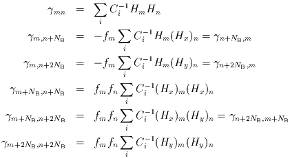
From Eqs. III.3.c.11 and III.3.c.13, the individual components of are given by:

(Eq. III.3.c.14-19)

The diagonal elements of the inverse of then correspond to lower limits for the variances of the estimated quantities, i.e.,

(Eq. III.3.c.20 - 22)

It can be shown that if the measurement model is linear, equality holds in the above expressions. Since the measurement model is linear in flux, equation 20 therefore yields realistic values for the flux uncertainties. In the case of the positional uncertainties, however, the above expressions provide lower limits only.

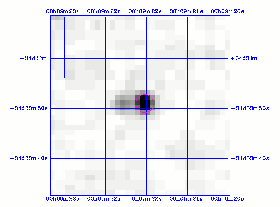
The blend number, N_B is specified in each record of the Point Source Catalog as ``bln_flg" (blend flag), and indicates the number of candidates fit simultaneously. Blend flag values >1 are therefore useful as indicators of possible confusion in regions of high source density. For example, Figure 1 shows the K_s image of sources 2MASSI J0009220+343350 and 2MASSI J0009260+335945. The former is the brighter of the two objects, and is a 3-band detection having a bln_flg of "112." The latter source is the fainter of the pair, is detected only in the H and K_s bands, and has a bln_flg of "012." Both sources are clearly visible in all three bands, but the pair was resolved only in H and K_s. The separation of the pair in K_s was small enough so that the profile fitting was run simultaneously on both sources (N_B=2), but in H the separation was large enough that the sources were fitting individually. The chi-squared value of the J-fit in the bright source is 6.35, indicating that the single psf-fit was poor.

Objects with valid profile-fit R2-R1 photometry (i.e., non-saturated and converged profile fit) have ``rd_flg'' values of ``2'' in the Point Source Catalog record. This corresponds to the great majority of all point sources in the Catalog.

Figure 1

Point Spread Functions and Seeing Estimation

The source contribution to the profile fit model is proportional to a point-spread-function (PSF) which is taken from a library of PSFs indexed by seeing for each band. PSF's are not derived "on-the-fly" during 2MASS pipeline processing because of the difficulty in automated PSF construction in much of the sky due to both very low and very high source density. PSF-derivation is also a cpu-intensive task, so the use of a PSF library results in much faster processing run times.

The library PSFs corresponding to specific seeing values were constructed empirically using from single 2MASS calibration scans having that average seeing value. Images of the 50 brightest stars in each scan are centroided and aligning, summed, and finally interpolated into a 0.1" grid. In addition to the PSFs themselves, an estimate of the uncertainty in the PSF (the "variance map") is also produced on the same grid and used by the profile fit analysis to estimate the total uncertainties in the resulting estimates. Selection of the calibration scans for PSF generation, and of the PSFs themselves, was based on criteria such as small variability of the seeing parameter during the scan, x- and y- central moments of the stars being equal (typically within 10%), and consistency with other PSFs taken under similar conditions. A single PSF is assumed to accurately characterize the point source profile across the 2MASS focal plane for the purposes of the data processing.

The appropriate PSF is chosen for the profile fitting photometry during the processing of a 2MASS survey scan by estimating the mean point source diameter (seeing) on spatial scales no finer than the length of an Atlas Image, 17', corresponding to a time interval in the scan of approximately 18 sec. The actual interval used to determine the seeing is driven by source density, and in low star density regions the interval can be up to 3 times longer. If the seeing is variable on timescales shorter than the seeing estimation response time, there can be a photometric error of up to several percent induced by a mismatch between the true image profile and the PSF used in profile-fitting photometry.

Aperture Photometry and Curve of Growth Correction

Aperture photometry is also performed for each candidate detection from the Atlas Images to provide a reference to the absolute photometric scale for the profile-fit photometry, statistics on the detectability of an object, and as a back-up source of brightness information when profile-fitting fails to converge to a valid measurement. As with the profile fitting, the aperture photometry is made at the position of the faint detections on the individual frames. The brightness is measured in a series of apertures ranging in radius from 3" to 14", in 1" steps, by summing pixels entirely within the aperture and interpolating pixels partially within the aperture. The sky background for each object is computed in an annulus with an inner radius of 14.0" and an outer radius of 20.0". Pixels in the sky annulus are entirely included or excluded based on the distance of their centers from the source. The sky value is estimated by first excluding saturated, masked, or unreasonably low pixels. A sigma-trimmed median of the surviving sky pixels is then used as the sky estimate. The aperture measurements from each of the six input frames are combined using an unweighted average. Aperture measurements are usually possible on six frames for each detection. However, if one of more of the frames contains a masked pixel within 4" of the source location, that frame is excluded from the the measurement. The aperture measurements from each of the remaining input frames are combined using an unweighted average. The "ndet_flg" parameter included in the Sampler Point Source Catalog record tabulates the number of frames on which a >3-sigma aperture photometry detection was made and the number of frames available for measurement, for each band of each source. For brighter sources, this can be used as a reliability indicator, and for fainter objects, it can be used as a sensitivity indicator.

The multiple aperture photometry for all sources observed under the same seeing conditions during a 2MASS survey scan is used to to determine the curve-of-growth correction to the aperture measurements. The curve-of-growth correction is defined to be the constant factor that when applied to "standard aperture" magnitudes (measured in the 4" radius aperture) makes them equivalent to an "infinite" size aperture. This accounts for any light that falls outside of this aperture without suffering from degraded signal-to-noise that would result from simply using the measurement from large apertures. The curve-of-growth correction is seeing dependent: when the seeing is poorer, the correction is larger. The curve-of-growth is evaluated by calculating the differences between successive aperture magnitudes for each R2-R1 source and testing for when the differences converge to zero, or when the differences begin to diverge, within measurement uncertainties. The correction is the median difference between the 4" aperture magnitude and the magnitude in the aperture at which the magnitude differentials become zero, for a large ensemble of stars.

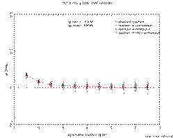
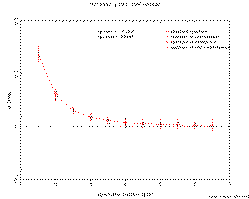
J-band curves-of-growth evaluated during periods of good (2.5" FWHM) and bad (3.4" FWHM) seeing in scans from the Spring 1999 Data Release are shown in Figure 2 and Figure 3, respectively. The x-axes show aperture radius in pixels (2"/pixel), and the y-axes show the difference between successive aperture magnitudes plotted versus the outer radius. Indicated on the figures are the radius of the "standard aperture" (open circle), and the radius at which the curve-of-growth was determined to converge (open star). The good seeing case shown in Figure 2, converges at a smaller radius, 2.5 pix, than the poor seeing case, 4.0 pix. The curve-of-growth correction determined in these examples were -0.016+0.005 mags and -0.121+0.015 mags, respectively.

The "default magnitude" given for most objects in the 2MASS Sampler Point Source Catalog is the profile-fit magnitude. The curve-of-growth-corrected "standard aperture" (4" radius) magnitudes (j_m_stdap, h_m_stdap and k_m_stdap) and uncertainties are also provided for most objects in the Point Source Catalog. On occasion, the profile-fitting photometry for a source will fail to converge, and no valid point-source photometry will be produced. If there exists a curve-of-growth-corrected aperture magnitude for such objects, this magnitude will be listed in the "default magnitude" entry, and the "rd_flg" for the appropriate band will have a value of "4." Extreme caution should be used in interpreting these magnitudes because they sources are usually found in confused regions where there is often serious contamination in the sky annuli for the aperture measurements.

Figure 2	Figure 3

Photometric Normalization

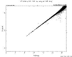
The point source profile-fit photometry is tied to the absolute photometric scale of the system by normalizing to the curve-of-growth-corrected aperture photometry. This is done separately for all sources in a survey scan having the same seeing value, since the normalization can change with seeing. The median offset between profile-fit and curve-of-growth-corrected aperture photometry is calculated iteratively with 3-sigma rejection for all stars. The resulting offset correction is added to the profile-fit photometry, and this corrected value is the "default magnitude" listed in the Point Source Catalog record for most sources ("rd_flg" = "2"). Figure 4 shows the relationship between profile-fit and curve-of-growth-corrected aperture magnitudes for a scan in the Spring 1999 Data Release, after the normalization correction has been applied to the profile-fit photometry. In some regions of very low source density, there are not enough sources to empirically determine the normalization. In these cases, a normalization factor is selected from a table indexed by the seeing.

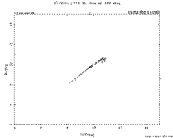
The R1 aperture photometry for all sources is then normalized to the corrected profile-fit photometry, using objects that are both bright enough to have been detected in the R1 frames but below the R2-R1 saturation limit, and therefore having valid profile-fit photometry. There is typically 2-3 magnitudes of overlap to provide an empirical measure of any offset between the photometric scales. As with the profile-fit/aperture photometry normalization, the median offset between the R1 aperture and corrected profile-fit photometry for all available sources is calculated iteratively using 3-sigma rejection. This correction is then applied to the R1 photometry for all sources, and the corrected magnitudes are listed in the "default magnitude" fields for the Sampler Point Source Catalog for all objects saturated in the R2-R1 exposures ("rd_flg" = "1"). Figure 5 shows the normalized R1 magnitudes plotted as a function of their equivalent corrected profile-fit magnitude for a night in the Spring 1999 Data Release. This figure also illustrates the overlap in the range over which both R1 and R2-R1 provide useful measurements. In low source density regions there may not be enough bright stars to allow measurement of the R1 normalization factor. In these cases, a pre-evaluated factor is selected froma table indexed by seeing.

Figure 4	Figure 5

Very Bright Stars

Stars brighter than approximately 4th to 5th magnitude will saturate in even the 51ms R1 exposures. The photometry algorithms are currently unable to evaluate useful magnitudes for these objects, so the default magnitudes are set to -99.999 in the Inremental PSC for any saturated bands. The corresponding "rd_flg" value for those bands is "3".

Very bright stars, 2-3 magnitudes brighter than the R1 saturation level, may not be unambiguously detected during the point source characterization. Placeholders for these very bright stars are included in the 2MASS Spring 1999 Point Source Catalog, with positions taken from external catalogs such as the Hipparcos, ACT, or PPM catalogs, when available. The decision to include a placeholders is based on photometric estimates for objects from the Catalog of Infrared Observations (Gezari, Schmitz & Meade 1987, NASA Publication 1196), and the Two Micron Sky Survey, or near infrared magnitudes deduced from visual and/or IRAS 12 micron photometry and some knowledge of the stellar spectral type. These placeholders are almost certainly incomplete in the Galactic plane. Because many of the brightest near infrared stars are variables, and because of large uncertainties in the interpolated magnitudes for the placeholders, there are instances of a placeholder being in the PSC when 2MASS has not detected a bright star at the location.

The "placeholder" entries in the PSC have "rd_flag" values of "8". The positions of these entries should be used only with extreme caution, and are provided for informational purposes only. There are 1730 very bright star placeholder entries in the 2MASS Spring 1999 PSC. The brightest star in the release area is probably the K5 giant alpha Tau (2MASSI J0435552+163034), with K~-2.9.

[Last Updated: 1999 May 5; by R. Cutri, E. Kopan, K. Marsh, T. Evans]