IV. 2MASS Data Processing

5. Extended Source Identification and Photometry

d. Improved Ellipse Fitting and Isophotal Photometry in Crowded Fields

The basic ellipse fitting algorithm is described in Jarrett et al. 2000. The following figures demonstrate an improved method by which to derive the 3- ellipse parameters of a galaxy, thus improving the photometry.

Neighboring stars both confuse the desired isophote (3 in this case) and systematically bump up the flux of a galaxy. The nominal GALWORKS solution to this dilemma is to mask all of the stars detected in the pipeline, derive the ellipse parameters from the chopped-up image, and recover the lost flux using isophotal substitution (i.e., assume symmetry and use the ellipse parameters to build a ellipsoid model of the galaxy).

The modifications are mostly subtle, but with one significant difference. Instead of masking the stars outright, the new method subtracts the stars. Before this subtraction can occur, however, the underlying galaxy itself must be subtracted. Hence, the method is to employ an iterative loop that searches for the ellipsoid model of the galaxy with star subtraction.

Method

1. Derive a first guess at the ellipse parameters of galaxy, i.e., axis ratio and position angle. Since nearby stars may distort the 3- isophote, the most reliable first guess is arrived at by using the inner 8´´ radius of the galaxy. Here we compute the axis ratio and position angle by computing the optimal second moment ratio (similar to what is already being used to derive the PSF elongation). The solution will be biased towards a more circular axis ratio, due to the round PSF, but the axis ratio will be close to the correct answer. Keep in mind this is only a crude first guess.

2. Using the first-guess axis ratio and position angle, subtract the galaxy from the image (using the centroid position of the galaxy). The subtraction is performed by computing the lower quartile flux in the elliptical annulus and subtracting this value from the image (i.e., build an ellipsoid using the lower quartile in each annulus of width 1 pixel). The lower quartile is most robust against stars.

3. Subtract stars from image (with the galaxy remaining intact). Here we use the galaxy-subtracted image to properly subtract the stars from the nominal image. The "subtraction" is carried out as follows: compute the median local "sky" value using an annulus about the star to be subtracted. Then, compute the difference between the untouched image and the local median value. It is this difference that represents the flux of the star. Subtract the difference from the untouched image. The subtraction is performed on a circular area containing the star. The size of the area depends on the brightness of the star, where we employ the generalized exponential function,
   f(dr) = f₀ * exp {-dr/)^(1/)]

   which nicely models the PSF. Here we need to know the "shape" or ( * ) and . The "shape" comes from SEEMAN (and GALWORKS), computed for every Atlas Image (hence, tracking the PSF seeing). The parameter also comes from GALWORKS, but for only the scan average.

   Here, we centroid the star to get the correct position. We use the peak flux of the source, f₀, corresponding to the peak of the galaxy-subtracted image.

   The subtraction is not fully completed, however. We use isophotal substitution (i.e., using the symmetric shape of the object; see step 4 below) as an additional component which is averaged with the resultant residual, described above.

4. We now derive the ellipse parameters for the 3- isophote of the star-subtracted image. We use the same method employed in GALWORKS.

5. Redo steps 2 through 4, using the latest, greatest ellipse model solution.

With the ellipse parameters optimally derived, we then can perform isophotal substitution to eliminate the stars from the photometry. Note: we could use the star-subtracted image; however, there will always be residual flux from the star, since subtraction is not perfect, particularly for the central pixels of the star. Isophotal substitution is probably the most robust method for eliminating stars; however, note that this only works if the galaxy is symmetric (which is usually the case).

Illustrations

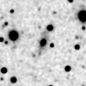
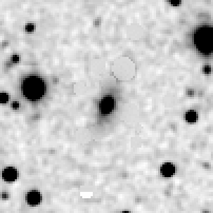
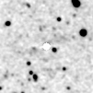
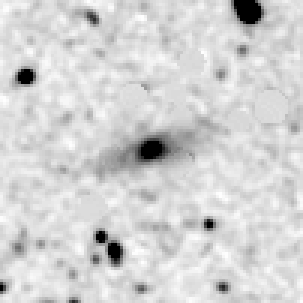
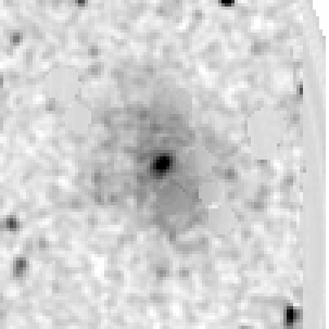
Case 1: galaxy at (ra, dec) = (241.9399, -59.92483), or (glon, glat) = (325.3076, -5.8810), with K_s=11 mag. The stellar density is high, at 4.16 (log no. sources deg^-2 brighter than K_s=14 mag). Figure 1 shows the K_s-band image, 101´´ × 101´´ field.

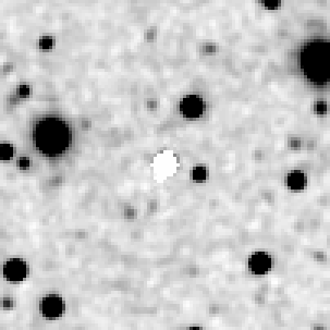
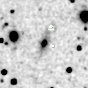
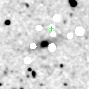
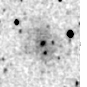
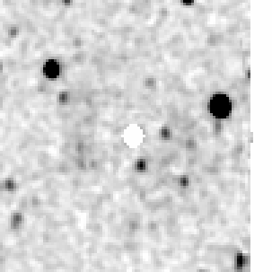
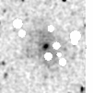
Figure 2 shows the galaxy subtracted using a symmetric ellipsoid model. The ellipse parameters are derived (using second moment): axis ratio = 0.778, p.a. = 160.0. Using the old method, masking stars, we obtain what is shown in Figure 3. Using the new method, locating and subtracting stars, we obtain what is shown in Figure 4.

Figure 1	Figure 2	Figure 3	Figure 4

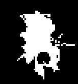
Using the old GALWORKS method, we derive the new ellipse parameters axis ratio = 0.520 and p.a. = 160.0. Figure 5 shows the "raw" isophote, and Figure 6 shows the solution. Using the new method, we obtain axis ratio = 0.360 and p.a. = 165.0. Figure 7 shows the "raw" isophote, and Figure 8 shows the solution.

Figure 5	Figure 6	Figure 7	Figure 8

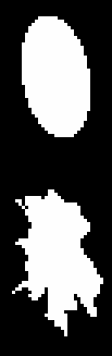
Next, we eliminate stars from original image using isophotal substitution. Figure 9 shows the results of the old method, while Figure 10 shows the results of the new method. Steps 2-4 are repeated using the new method (note that the images and solutions shown above are for the second iteration). With the new method we arrive at a final solution that is closer to "truth" than with the nominal, old method.

Figure 9	Figure 10

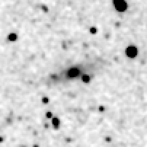
Case 2: galaxy at (ra, dec) = (241.82357, -60.68036), or (glon, glat) = (324.7513, -6.3989), with K_s=10.8 mag. The stellar density is 4.1. Figure 11 shows the K_s-band image, 101´´ × 101´´ field.

Figure 12 shows the galaxy subtracted using a symmetric ellipsoid model. The ellipse parameters are derived (using second moment): axis ratio = 0.7650, p.a. = 94.0. Using the old method, masking stars, we obtain what is shown in Figure 13. Using the new method, locating and subtracting stars, we obtain what is shown in Figure 14.

Figure 11	Figure 12	Figure 13	Figure 14

Using the old GALWORKS method, we derive the new ellipse parameters axis ratio = 0.340, p.a. = 105.0. Figure 15 shows the "raw" isophote, and Figure 16 shows the solution. Using the new method, we obtain axis ratio = 0.360, p.a. = 108.0. Figure 17 shows the "raw" isophote, and Figure 18 shows the solution.

Figure 15	Figure 16	Figure 17	Figure 18

Next, we eliminate stars from original image using isophotal substitution. Figure 19 shows the results of the old method, while Figure 20 shows the results of the new method. Repeat steps 2-4 for the new method, etc.

Figure 19	Figure 20

Case 3: face-on late-type galaxy at (ra,dec) = (284.901672, 19.427221), or (glon, glat) = (51.2129, 6.9933), with K_s=10.3 mag. The stellar density is 3.85. (This is perhaps the "worst-case scenario.") Figure 21 shows the K_s-band image, 101´´ × 101´´ field.

Figure 22 shows the galaxy subtracted using a symmetric ellipsoid model. The ellipse parameters are derived (using second moment): axis ratio = 0.9843, p.a. = 6.0. Using the old method, masking stars, we obtain what is shown in Figure 23. Using the new method, locating and subtracting stars, we obtain what is shown in Figure 24.

Figure 21	Figure 22	Figure 23	Figure 24

Using the old GALWORKS method, we derive the new ellipse parameters, axis ratio = 0.480, p.a. = 10.0. Figure 25 shows the "raw" isophote, and Figure 26 shows the solution. Using the new method, we obtain axis ratio = 0.540, p.a. = 10.0. Figure 27 shows the "raw" isophote, and Figure 28 shows the solution.

Figure 25	Figure 26	Figure 27	Figure 28

Next, we eliminate stars from original image using isophotal substitution. Figure 29 shows the results of the old method, while Figure 30 shows the results of the new method. Repeat steps 2-4 for the new method, etc.

Figure 29	Figure 30

Axis Ratio and Small Radii

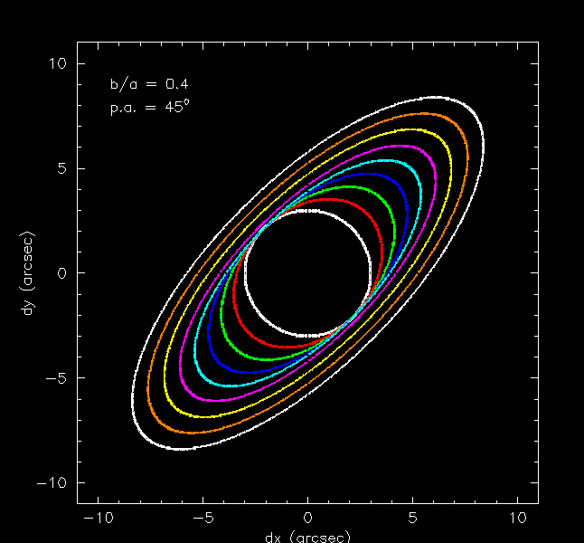
Finally, for small radii, we adjust the axis ratio such that the minimum semi-minor axis is 3´´. This modification is needed to counteract the circularizing effects of the PSF. The half-light "effective" aperture and Kron aperture are particularly affected by this modification, since they are allowed to shrink to radii near the PSF.

An example of a dynamically adjusted axis ratio is shown in Figure 31. The nominal axis ratio is 0.4, and the position angle is -45°. Note the increasingly circular aperture, as the radius approaches the size of the PSF.

Figure 31

[Last Updated: 2002 Jul 15; by T. Jarrett]